Order Analysis of a Vibration Signal
This example shows how to analyze a vibration signal using order analysis. Order analysis is used to quantify noise or vibration in rotating machinery whose rotational speed changes over time. An order refers to a frequency that is a certain multiple of a reference rotational speed. For example, a vibration signal with a frequency equal to twice the rotational frequency of a motor corresponds to an order of two and, likewise, a vibration signal that has a frequency equal to 0.5 times the rotational frequency of the motor corresponds to an order of 0.5. In this example, orders of large amplitude are determined to investigate the source of unwanted vibration in a helicopter cabin.
Introduction
This example analyzes simulated vibration data from an accelerometer in the cabin of a helicopter during a run-up and coast-down of the main motor. A helicopter has several rotating components, including the engine, gearbox, and the main and tail rotors. Each component rotates at a known, fixed rate with respect to the main motor, and each may contribute to unwanted vibration. The frequency of dominant vibration components can be related to the rotational speed of the motor to investigate the source of high-amplitude vibration. The helicopter in this example has four blades in both the main and tail rotors. Important components of vibration from a helicopter rotor may be found at integer multiples of the rotational frequency of the rotor when the vibration is generated by the rotor blades.
The signal in this example is a time-dependent voltage, vib, sampled at a rate fs equal to 500 Hz. The data include rpm, the angular speed of the turbine engine, and a vector t of time instants. The ratio of rotor speed to engine speed for each rotor is stored in the variables mainRotorEngineRatio and tailRotorEngineRatio.
A motor speed signal commonly consists of a sequence of tachometer pulses. tachorpm can be used to extract an RPM signal from a tachometer pulse signal. tachorpm automatically identifies the pulse locations of a bilevel tachometer waveform and computes the interval between pulses to estimate rotational speed. In this example, the motor speed signal contains the rotational speed, rpm, and hence no conversion is needed.
Plot the motor speed and vibration data as functions of time:
load helidata
vib = vib - mean(vib);  % Remove the DC component

subplot(2,1,1)
plot(t,rpm)             % Plot the engine rotational speed
xlabel('Time (s)')
ylabel('Engine Speed (RPM)')
title('Engine speed')

subplot(2,1,2)
plot(t,vib)             % Plot the vibration signal
xlabel('Time (s)')
ylabel('Voltage (mV)')
title('Accelerometer Vibration Data')
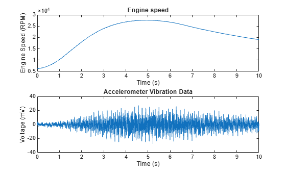
The engine speed increases during the run-up and decreases during the coast-down. The vibration amplitude changes as a function of rotational speed. This type of RPM profile is typical for analyzing vibration in rotating machinery.
Visualizing Data Using An RPM-Frequency Map
The vibration signal can be visualized in the frequency domain using the function rpmfreqmap. This function computes the short-time Fourier transform of the signal and generates an RPM-frequency map. rpmfreqmap displays the map in an interactive plot window when output arguments are omitted.
Generate and visualize an RPM-frequency map for the vibration data.
rpmfreqmap(vib,fs,rpm)
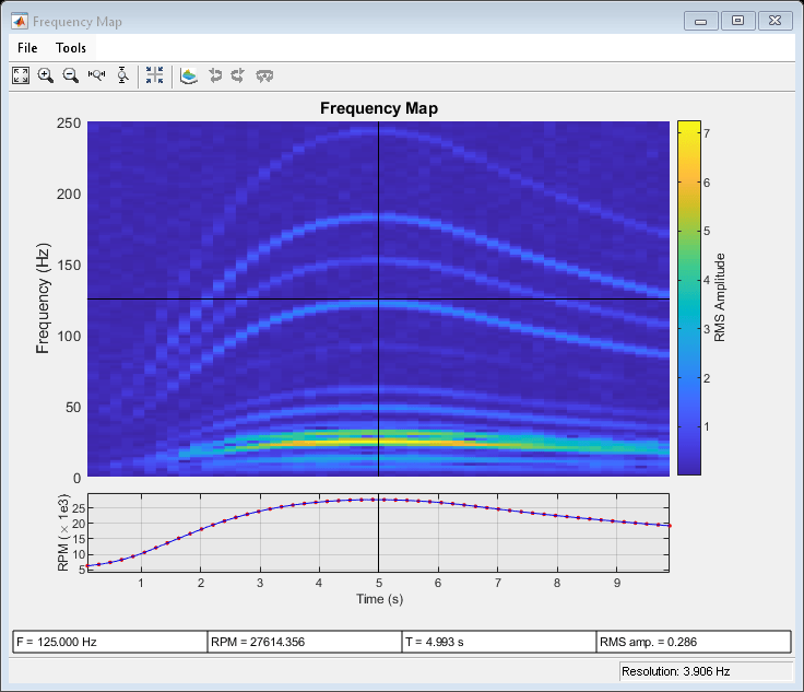
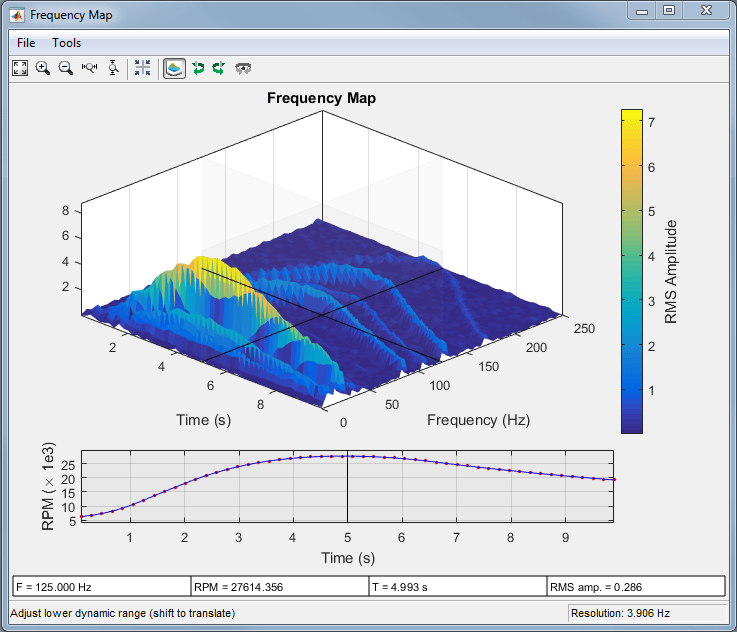
The interactive figure window produced by rpmfreqmap contains an RPM-frequency map, an RPM versus time curve corresponding to the map, and several numeric indicators that can be used to quantify vibration components. The amplitude of the map represents root-mean-square (RMS) amplitude by default. Other amplitude choices, including peak amplitude and power, can be specified with optional arguments. The waterfall plot menu button generates a three-dimensional view:
Many of the tracks in the RPM-frequency maps have frequencies that increase and decrease with the motor speed. This suggests that the tracks are orders of the motor rotational frequency. There are high-amplitude components near the RPM peak, with frequencies between 20 and 30 Hz. The crosshair cursor can be placed on the map at this location to view the frequency, RPM value, time, and map amplitude in the indicator boxes below the RPM curve.
By default, rpmfreqmap computes the resolution by dividing the sample rate by 128. The resolution is displayed in the lower-right corner of the figure, and is equal to 3.906 Hz in this case. A Hann window is used by default, but several other windows are available.
Pass a smaller the value of the resolution to rpmfreqmap to resolve certain frequency components better. For example, low-frequency components are not separated at the peak RPM. At low RPM values, the high-amplitude tracks appear to blend together.
Generate an RPM-frequency map with a resolution of 1 Hz to resolve these components.
rpmfreqmap(vib,fs,rpm,1)
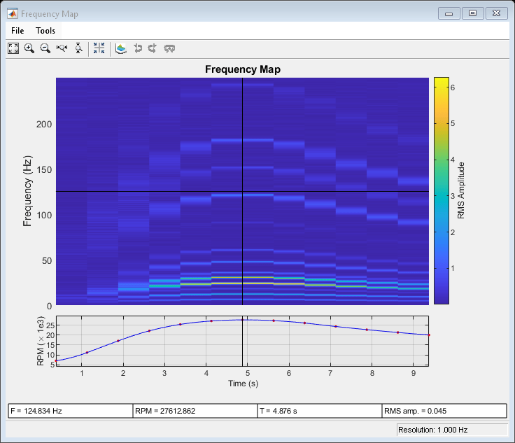
Low-frequency components can now be resolved at the peak RPM, but there is significant smearing present when the rotational speed is changing more rapidly. Vibration orders change frequency within each time window as the motor speed increases or decreases, producing a broader spectral track. This smearing effect is more pronounced for a finer resolution because of the longer time windows that are required. In this case, improving the spectral resolution resulted in increased smearing artifacts during the run-up and coast-down phases. An order map can be generated to avoid this trade-off.
Visualizing Data Using An RPM-Order Map
The function rpmordermap generates a spectral map of order versus RPM for order analysis. The approach removes smearing artifacts by resampling the signal at constant phase increments, producing a stationary sinusoid for each order. The resampled signal is analyzed using a short-time Fourier transform. Since each order is a fixed multiple of the reference rotational speed, an order map contains a straight order track as a function of RPM for each order.
The function rpmordermap accepts the same arguments as rpmfreqmap and also produces an interactive plot window when called with no output arguments. The resolution parameter is now specified in orders, rather than in Hz, and the spectral axis of the map is now order, rather than frequency. The function uses a flat-top window by default.
Visualize the order map of the helicopter data using rpmordermap. Specify an order resolution of 0.005 orders.
rpmordermap(vib,fs,rpm,0.005)
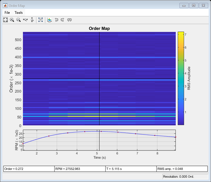
The map contains a straight track for each order, indicating that the vibration occurs at a fixed multiple of the motor rotational speed. Order maps make it easy to relate each spectral component to the motor speed. Smearing artifacts are significantly reduced compared to the RPM-frequency map.
Determining Peak Orders Using an Average Order Spectrum
Next, determine the locations of the peaks of the order map. Look for orders that are integer multiples of the order of the main and tail rotors, where vibration generated by these rotors would occur. The function rpmordermap returns the map and corresponding order and RPM values as outputs. Analyze the data to determine the orders of high-amplitude vibration in the helicopter cabin.
Compute and return an order map of the data.
[map,mapOrder,mapRPM,mapTime] = rpmordermap(vib,fs,rpm,0.005);
Next, use orderspectrum to compute and plot the average spectrum of map. The function takes the order map generated by rpmordermap as input and averages it over time.
figure
orderspectrum(map,mapOrder)
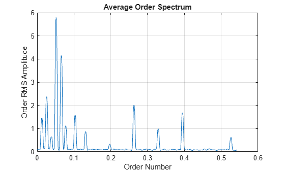
Return the average spectrum and call findpeaks to return the locations of the two highest peaks.
[spec,specOrder] = orderspectrum(map,mapOrder);
[~,peakOrders] = findpeaks(spec,specOrder,'SortStr','descend','NPeaks',2);
peakOrders = round(peakOrders,3)
peakOrders = 2×1

    0.0520
    0.0660
Two closely spaced dominant peaks can be seen around order 0.05 in the plot. The orders are less than one because the frequency of vibration is lower that the rotational speed of the motor.
Analyzing Peak Orders Over Time
Next, find the amplitudes of the peak orders as a function of time using ordertrack. Use map as an input and plot the amplitude of the two peak orders by calling ordertrack with no output arguments.
ordertrack(map,mapOrder,mapRPM,mapTime,peakOrders)
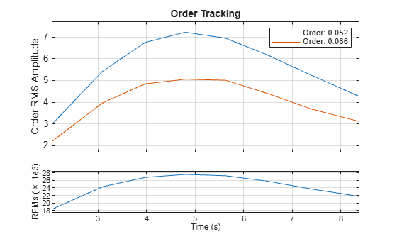
Both orders increase in amplitude as the rotational speed of the motor increases. Although orders can be easily separated in this case, ordertrack can also separate crossing orders when multiple RPM signals are present.
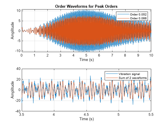
Next, extract a time-domain order waveform for each peak order using orderwaveform. Order waveforms can be compared directly to the original vibration signal and played back as audio. orderwaveform uses the Vold-Kalman filter to extract order waveforms for specified orders. Compare the sum of two peak-order waveforms to the original signal.
orderWaveforms = orderwaveform(vib,fs,rpm,peakOrders);
helperPlotOrderWaveforms(t,orderWaveforms,vib)
Reducing Cabin Vibration
To identify the sources of the cabin vibration, compare the order of each peak to the order of each of the helicopter's rotors. The order of each rotor is equal to the fixed ratio of the rotor speed to the engine speed.
mainRotorOrder = mainRotorEngineRatio;
tailRotorOrder = tailRotorEngineRatio;

ratioMain = peakOrders/mainRotorOrder
ratioMain = 2×1

    4.0310
    5.1163
ratioTail = peakOrders/tailRotorOrder
ratioTail = 2×1

    0.7904
    1.0032
The highest peak is located at order four of the main rotor speed, so the frequency of the maximum-amplitude component is four times the frequency of the main rotor. The main rotor, which has four blades, is a good candidate for the source of this vibration because, for a helicopter with N blades per rotor, vibration at N times the rotor rotational speed is common. Likewise, the second largest component is located at order one of the tail rotor speed, suggesting vibration may originate from the tail rotor. Because the speeds of the rotors are not related by an integer factor, the order of the second largest peak with respect to the main rotor speed is not an integer.
After making track and balance adjustments to the main and tail rotors, a new data set is collected. Load it and compare the order spectra before and after the adjustment.
load helidataAfter
vib = vib - mean(vib);             % Remove the DC component
[mapAfter,mapOrderAfter] = rpmordermap(vib,fs,rpm,0.005);
figure
hold on
orderspectrum(map,mapOrder)
orderspectrum(mapAfter,mapOrderAfter)
legend('Before Adjustment','After Adjustment')
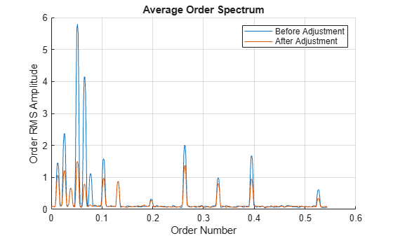
The amplitudes of the dominant peaks are now considerably lower.
Conclusions
This example used order analysis to identify the main and tail rotors of a helicopter as potential sources of high-amplitude vibration in the cabin. First, rpmfreqmap and rpmordermap were used to visualize orders. The RPM-order map provided order separation throughout the RPM range without the smearing artifacts present in the RPM-frequency map. rpmordermap was the best choice to visualize vibration components at lower RPM during the engine run-up and coast-down.
Next, the example used orderspectrum to identify peak orders, ordertrack to visualize the amplitude of the peak orders over time, and orderwaveform to extract time-domain waveforms for the peak orders. The order of the largest amplitude vibration component was found at four times the rotational frequency of the main rotor, indicating an imbalance in the main rotor blades. The second largest component was found at the rotational frequency of the tail rotor. Adjustments to the rotors resulted in reduced vibration levels.
References
Brandt, Anders. Noise and Vibration Analysis: Signal Analysis and Experimental Procedures. Chichester, UK: John Wiley and Sons, 2011.
See Also
orderspectrum | ordertrack | orderwaveform | rpmfreqmap | rpmordermap
You can also select a web site from the following list:
Americas
- América Latina (Español)
- Canada (English)
- United States (English)
Europe
- Belgium (English)
- Denmark (English)
- Deutschland (Deutsch)
- España (Español)
- Finland (English)
- France (Français)
- Ireland (English)
- Italia (Italiano)
- Luxembourg (English)
- Netherlands (English)
- Norway (English)
- Österreich (Deutsch)
- Portugal (English)
- Sweden (English)
- Switzerland
- United Kingdom (English)