Tire Parameterization and Performance
This example shows how to use Simscape™ Driveline™ to fit tire Magic Formula coefficients to experimental data and to measure the simulated stopping distance of a vehicle supported by the tires. The example uses the sdlUtility.tirread function to load initial tire parameters from a .TIR file. Then, the example uses the MATLAB® optimization function fminsearch with a test harness model to fit the tire coefficients to the experimental data. Other products available for performing this type of parameter fitting with Simscape Driveline models are the Optimization Toolbox™ and Simulink® Design Optimization™. These products provide predefined functions to manipulate and analyze blocks using GUIs or a command line approach. This example uses Fast Restart to quickly simulate tire response for different parameters during the optimization.
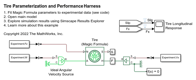
Model
The model contains a simple vehicle body supported by four tires. An Ideal Torque Source and two Disk Friction Clutch blocks specify the wheel torque conditions. The test scenario in this example accelerates and then brakes the vehicle.

Optimization Procedure and Results
This example considers 14 Magic Formula coefficients that affect the tire longitudinal force-slip behavior. The parameter fit procedure uses a test harness model that drives a tire with the same vertical load, rotational velocity, and longitudinal velocity as the experimental data. An Ideal Force Sensor measures the longitudinal force of the tire. The optimization objective function considers the least squares error between the simulated and experimentally measured longitudinal forces. The model uses Fast Restart to keep the model compiled between optimization iterations.
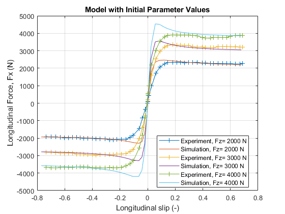
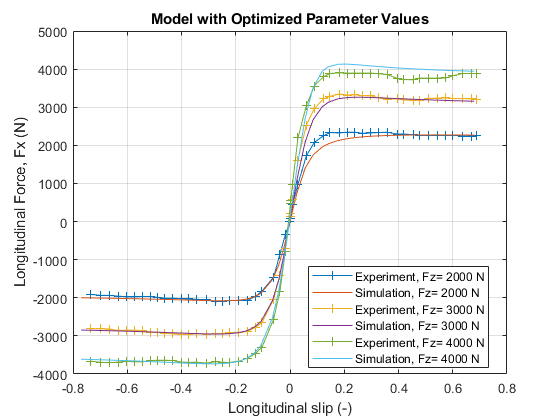
This example fits the Magic Formula longitudinal coefficients to experimental data provided in A. Ortiz, J. Cabrera, A. Guerra, and A. Simon, An easy procedure to determine Magic Formula parameters: A comparative study between the starting value optimization technique and IMMa optimization algorithm Vehicle System Dynamics. Taylor & Francis, 2006. The optimization procedure initializes the 14 coefficients with guessed values. The first figure below shows the mismatch between the initial tire longitudinal force-slip characteristics and the experimental data. The second figure shows closer agreement after the parameter optimization. Since fminsearch is an unconstrained nonlinear optimizer that locates a local minimum of a function, varying the initial estimate will result in a different solution set.
Initial coefficient values are:
	P_Cx1 =   1.397
	P_Dx1 =     1.1
	P_Dx2 =  -0.182
	P_Ex1 =  -0.459
	P_Ex2 =    -1.5
	P_Ex3 =   0.006
	P_Ex4 =   -0.91
	P_Kx1 =      38
	P_Kx2 =   2.031
	P_Kx3 =    -0.6
	P_Hx1 = -0.0017
	P_Hx2 =   0.003
	P_Vx1 =   0.057
	P_Vx2 =   -0.03
Optimized coefficient values are:
	P_Cx1 =     1.26268
	P_Dx1 =    0.977901
	P_Dx2 =   -0.209517
	P_Ex1 =   -0.487528
	P_Ex2 =    -1.63709
	P_Ex3 =  0.00638911
	P_Ex4 =    -1.06055
	P_Kx1 =     14.2857
	P_Kx2 =     2.12097
	P_Kx3 =   -0.539739
	P_Hx1 = -0.00208473
	P_Hx2 =   0.0032325
	P_Vx1 =    0.063874
	P_Vx2 =  -0.0273162
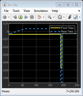
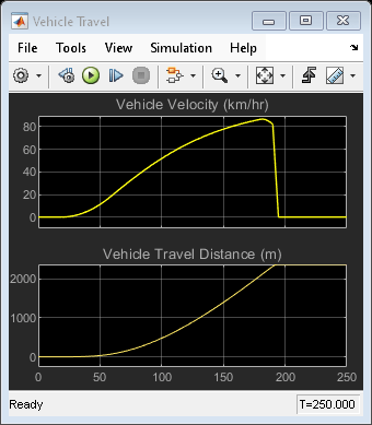
Simulation Results from Scopes
The scopes show vehicle velocity and travel distance, as well as front and rear tire slip. Tire slip spikes when the brakes are first applied.
Simulation Results from Simscape Logging
This plot shows the vehicle velocity versus travel distance. The markers indicate when the brake is first engaged and when the vehicle comes to a stop. With these vehicle and tire parameters, the vehicle has a stopping distance of approximately 44 meters when braking starts at a vehicle velocity of 21 meters per second.