Modeling for Single-Tasking Execution
Single-Tasking Mode
You can execute model code in a strictly single-tasking manner. While this mode is less efficient with regard to execution speed, in certain situations, it can simplify your model.
In single-tasking mode, the base sample rate must define a time interval that is long enough to allow the execution of all blocks within that interval.
The next figure illustrates the inefficiency inherent in single-tasking execution.

Single-tasking system execution requires a base sample rate that is long enough to execute one step through the entire model.
Build a Program for Single-Tasking Execution
To use single-tasking execution, clear model configuration parameter Treat each discrete rate as a separate task. If you select the parameter, single-tasking mode is used in the following cases:
If your model contains one sample time
If your model contains a continuous and a discrete sample time and the fixed step size is equal to the discrete sample time
Single-Tasking Execution
You can simulate and execute code generated from this simple multirate model, which is configured to use a fixed-step solver, in single-tasking or multitasking mode.
The tasking mode that gets applied depends on the setting of model configuration parameter Treat each discrete rate as a separate task. When cleared, the parameter specifies single-tasking mode. When selected, the parameter specifies multitasking mode.
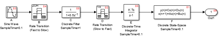
The example description refers to the six blocks in the model as A through F.
The execution order of the blocks (indicated in the upper right of each block) is forced into the order shown by assigning higher priorities to blocks F, E, and D. The ordering shown is one possible valid execution ordering for this model. For more information, see Simulation Phases in Dynamic Systems.
The execution order is determined by data dependencies between blocks. In a real-time system, the execution order determines the order in which blocks execute within a given time interval or task. This discussion treats the model execution order as a given, because it is concerned with the allocation of block computations to tasks, and the scheduling of task execution.
Note
The discussion and timing diagrams in this section are based on the assumption that the Rate Transition blocks are used in the default (protected) mode, with block parameters Ensure data integrity during data transfer and Ensure deterministic data transfer (maximum delay) selected.
When a model is configured for single-tasking execution and you select model configuration parameter Block reduction, fast-to-slow Rate Transition blocks are optimized out of the model. For this example, Block reduction is selected. Therefore, block B does not appear in the timing diagrams below. For more information, see Block reduction.
For each block in the model, this table shows the execution order, sample time, and whether the block has an output or update computation. Blocks A does not have an update computation because the block does not have discrete states.
Blocks | Sample Time | Output | Update |
|---|---|---|---|
E | 0.1 | Y | Y |
F | 0.1 | Y | Y |
D | 1 | Y | Y |
A | 0.1 | Y | N |
C | 1 | Y | Y |
Real-Time Single-Tasking Execution
This figure shows the scheduling of computations when the generated code is deployed in a real-time system in single-tasking mode. The generated program runs in real time under control of interrupts from a 10 Hz timer.

At time 0.0, 1.0, and every second thereafter, the slow and fast blocks execute output computations followed by update computations for blocks that have states. Within a given time interval, output and update computations are sequenced in block execution order.
The fast blocks execute on every tick, at intervals of 0.1 second. Output computations are followed by update computations.
The system spends some portion of each time interval (labeled “wait”) idling. During the intervals when only the fast blocks execute, a larger portion of the interval is spent idling. This illustrates an inherent inefficiency of single-tasking mode.
Simulated Single-Tasking Execution
This figure shows the execution of the model during a Simulink® simulation loop.

Because time is simulated, the placement of ticks represents the iterations of the simulation loop. Blocks execute in the same order as in the previous figure, but without the constraint of a real-time clock. Idle time is not present between simulated sample periods.
Related Topics
You can also select a web site from the following list:
Americas
- América Latina (Español)
- Canada (English)
- United States (English)
Europe
- Belgium (English)
- Denmark (English)
- Deutschland (Deutsch)
- España (Español)
- Finland (English)
- France (Français)
- Ireland (English)
- Italia (Italiano)
- Luxembourg (English)
- Netherlands (English)
- Norway (English)
- Österreich (Deutsch)
- Portugal (English)
- Sweden (English)
- Switzerland
- United Kingdom (English)