Simultaneous Stabilization Using Robust Control
This example uses the Robust Control Toolbox™ commands ucover and musyn to design a high-performance controller for a family of unstable plants.
Plant Uncertainty
The nominal plant model consists of a first-order unstable system.
Pnom = tf(2,[1 -2]);
The family of perturbed plants are variations of Pnom. All plants have a single unstable pole but the location of this pole varies across the family.
p1 = Pnom*tf(1,[.06 1]);              % extra lag
p2 = Pnom*tf([-.02 1],[.02 1]);       % time delay
p3 = Pnom*tf(50^2,[1 2*.1*50 50^2]);  % high frequency resonance
p4 = Pnom*tf(70^2,[1 2*.2*70 70^2]);  % high frequency resonance
p5 = tf(2.4,[1 -2.2]);                % pole/gain migration
p6 = tf(1.6,[1 -1.8]);                % pole/gain migration
Covering the Uncertain Model
For feedback design purposes, we need to replace this set of models with a single uncertain plant model whose range of behaviors includes p1 through p6. This is one use of the command ucover. This command takes an array of LTI models Parray and a nominal model Pnom and models the difference Parray-Pnom as multiplicative uncertainty in the system dynamics.
Because ucover expects an array of models, use the stack command to gather the plant models p1 through p6 into one array.
Parray = stack(1,p1,p2,p3,p4,p5,p6);
Next, use ucover to "cover" the range of behaviors Parray with an uncertain model of the form
P = Pnom * (1 + Wt * Delta)
where all uncertainty is concentrated in the "unmodeled dynamics" Delta (a ultidyn object). Because the gain of Delta is uniformly bounded by 1 at all frequencies, a "shaping" filter Wt is used to capture how the relative amount of uncertainty varies with frequency. This filter is also referred to as the uncertainty weighting function. Try a 4th-order filter Wt for this example:
orderWt = 4;
Parrayg = frd(Parray,logspace(-1,3,60));
[P,Info] = ucover(Parrayg,Pnom,orderWt,'InputMult');
The resulting model P is a single-input, single-output uncertain state-space (USS) object with nominal value Pnom.
P
Uncertain continuous-time state-space model with 1 outputs, 1 inputs, 5 states.
The model uncertainty consists of the following blocks:
  Parrayg_InputMultDelta: Uncertain 1x1 LTI, peak gain = 1, 1 occurrences
Model Properties

Type "P.NominalValue" to see the nominal value and "P.Uncertainty" to interact with the uncertain elements.
tf(P.NominalValue)
ans =

    2
  -----
  s - 2

Continuous-time transfer function.
Model Properties
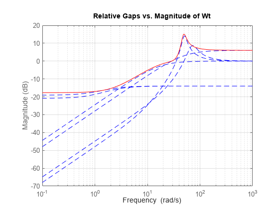
A Bode magnitude plot confirms that the shaping filter Wt "covers" the relative variation in plant behavior. As a function of frequency, the uncertainty level is 30% at 5 rad/sec (-10dB = 0.3) , 50% at 10 rad/sec, and 100% beyond 29 rad/sec.
Wt = Info.W1;
bodemag((Pnom-Parray)/Pnom,'b--',Wt,'r')
grid on
title('Relative Gaps vs. Magnitude of Wt')
Creating the Open-loop Design Model
To design a robust controller for the uncertain plant model P, we choose a desired closed-loop bandwidth and minimize the sensitivity to disturbances at the plant output. The control structure is shown below. The signals d and n are the load disturbance and measurement noise. The controller uses a noisy measurement of the plant output y to generate the control signal u.
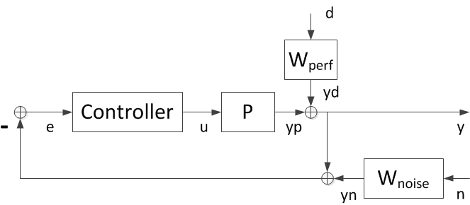
Figure 1: Control Structure.
The filters Wperf and Wnoise are selected to enforce the desired bandwidth and some adequate roll-off. The closed-loop transfer function from [d;n] to y is
y = [Wperf * S , Wnoise * T] [d;n]
where S=1/(1+PC) and T=PC/(1+PC) are the sensitivity and complementary sensitivity functions. If we design a controller that keeps the closed-loop gain from [d;n] to y below 1, then
|S| < 1/|Wperf| , |T| < 1/|Wnoise|
By choosing appropriate magnitude profiles for Wperf and Wnoise, we can enforce small sensitivity (S) inside the bandwidth and adequate roll-off (T) outside the bandwidth.
For example, choose Wperf as a first-order low-pass filter with a DC gain of 500 and a gain crossover at the desired bandwidth desBW:
desBW = 4.5;
Wperf = makeweight(500,desBW,0.33);
tf(Wperf)
ans =

  0.33 s + 4.248
  --------------
   s + 0.008496

Continuous-time transfer function.
Model Properties
Similarly, pick Wnoise as a second-order high-pass filter with a magnitude of 1 at 10*desBW. This will force the open-loop gain PC to roll-off with a slope of -2 for frequencies beyond 10*desBW.
NF = (10*desBW)/20;  % numerator corner frequency
DF = (10*desBW)*50;  % denominator corner frequency
Wnoise = tf([1/NF^2  2*0.707/NF  1],[1/DF^2  2*0.707/DF  1]);
Wnoise = Wnoise/abs(freqresp(Wnoise,10*desBW))
Wnoise =

    0.1975 s^2 + 0.6284 s + 1
  ------------------------------
  7.901e-05 s^2 + 0.2514 s + 400

Continuous-time transfer function.
Model Properties
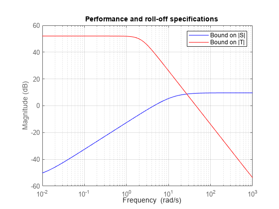
Verify that the bounds 1/Wperf and 1/Wnoise on S and T do enforce the desired bandwidth and roll-off.
bodemag(1/Wperf,'b',1/Wnoise,'r',{1e-2,1e3})
grid on
title('Performance and roll-off specifications')
legend('Bound on |S|','Bound on |T|','Location','NorthEast');
Next use connect to build the open-loop interconnection (block diagram in Figure 1 without the controller block). Specify each block appearing in Figure 1, name the signals coming in and out of each block, and let connect do the wiring:
P.u = 'u';
P.y = 'yp';
Wperf.u = 'd';
Wperf.y = 'Wperf';
Wnoise.u = 'n';
Wnoise.y = 'Wnoise';
S1 = sumblk('e = -ym');
S2 = sumblk('y = yp + Wperf');
S3 = sumblk('ym = y + Wnoise');
G = connect(P,Wperf,Wnoise,S1,S2,S3,{'d','n','u'},{'y','e'});
G is a 3-input, 2-output uncertain system suitable for robust controller synthesis with musyn.
Robust Controller Synthesis
The design is carried out with the automated robust design command musyn. The target bandwidth is 4.5 rad/s.
ny = 1; nu = 1;
[C,muPerf] = musyn(G,ny,nu);
D-K ITERATION SUMMARY:
-----------------------------------------------------------------
                       Robust performance               Fit order
-----------------------------------------------------------------
  Iter         K Step       Peak MU       D Fit             D
    1           353.6        249.5        251.9             0
    2           70.74        9.964        10.05             4
    3            1.98        1.604        1.621             8
    4           1.164        1.164        1.188            10
    5           1.091        1.091          1.1            10
    6           1.048        1.048        1.054            10
    7           1.028        1.028        1.034            10
    8           1.018        1.018        1.026            10
    9           1.014        1.014        1.017             8
   10           1.011        1.011        1.012             8

Best achieved robust performance: 1.01
When the robust performance indicator muPerf is near 1, the controller achieves the target closed-loop bandwidth and roll-off. As a rule of thumb, if muPerf is less than 0.85, then the performance can be improved upon, and if muPerf is greater than 1.2, then the desired closed-loop bandwidth is not achievable for the specified plant uncertainty.
Here muPerf is approximately 1 so the objectives are met. The resulting controller C has 18 states:
size(C)
State-space model with 1 outputs, 1 inputs, and 16 states.
You can use the reduce and musynperf commands to simplify this controller. Compute approximations of orders 1 through 17.
NxC = order(C);
Cappx = reduce(C,1:NxC);
For each reduced-order controller, use musynperf to compute the robust performance indicator and compare it with muPerf. Keep the lowest-order controller with performance no worse than 1.05 * muPerf, a performance degradation of 5% or less.
for k=1:NxC
   Cr = Cappx(:,:,k);  % controller of order k
   bnd = musynperf(lft(G,Cr));
   if bnd.UpperBound < 1.05 * muPerf
      break % abort with the first controller meeting the performance goal
   end
end

order(Cr)
ans =
6
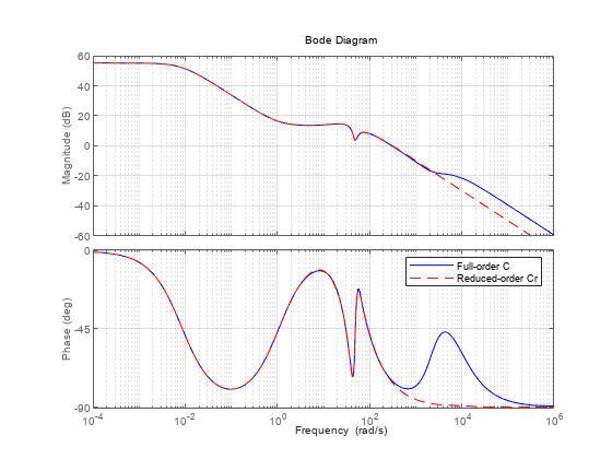
This yields a 6th-order controller Cr with comparable performance. Compare Cr with the full-order controller C.
bp = bodeplot(C,'b',Cr,'r--')
bp =
  BodePlot (Bode Diagram) with properties:

                 Responses: [2×1 controllib.chart.response.BodeResponse]
           Characteristics: [1×1 controllib.chart.options.CharacteristicsManager]

      PhaseWrappingEnabled: off
       PhaseWrappingBranch: -180
      PhaseMatchingEnabled: off
    PhaseMatchingFrequency: 0
        PhaseMatchingValue: 0
        MinimumGainEnabled: off
          MinimumGainValue: 0
          MagnitudeVisible: on
              PhaseVisible: on
                 PhaseUnit: "deg"
            MagnitudeScale: "linear"
             MagnitudeUnit: "dB"
            FrequencyScale: "log"
             FrequencyUnit: "rad/s"

                   Visible: on

  Show all properties
bp.PhaseMatchingEnabled = 'on';
legend('Full-order C','Reduced-order Cr','Location','NorthEast');
grid on
Robust Controller Validation
Plot the open-loop responses of the plant models p1 through p6 with the simplified controller Cr.
bp2 = bodeplot(Parray*Cr,'g',{1e-2,1e3})bp2 =
BodePlot (Bode Diagram) with properties:
Responses: [1×1 controllib.chart.response.BodeResponse]
Characteristics: [1×1 controllib.chart.options.CharacteristicsManager]
PhaseWrappingEnabled: off
PhaseWrappingBranch: -180
PhaseMatchingEnabled: off
PhaseMatchingFrequency: 0
PhaseMatchingValue: 0
MinimumGainEnabled: off
MinimumGainValue: 0
MagnitudeVisible: on
PhaseVisible: on
PhaseUnit: "deg"
MagnitudeScale: "linear"
MagnitudeUnit: "dB"
FrequencyScale: "log"
FrequencyUnit: "rad/s"
Visible: on
Show all properties
bp2.PhaseMatchingEnabled = 'on';
grid on
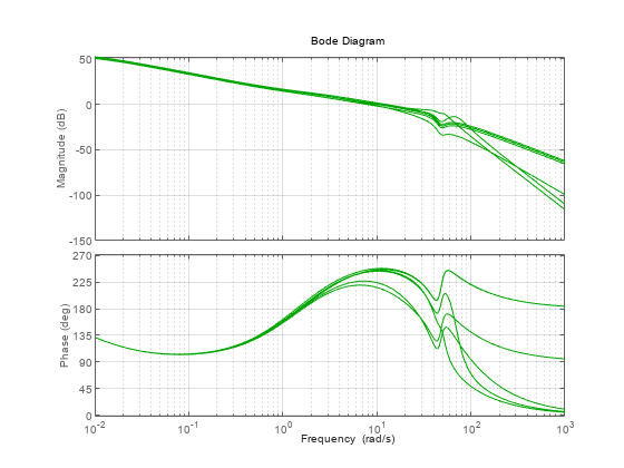
Plot the responses to a step disturbance at the plant output. These are consistent with the desired closed-loop bandwidth and robust to the plant variations, as expected from a Robust Performance mu-value of approximately 1.
stepplot(feedback(1,Parray*Cr),'g',10/desBW);
Varying the Target Closed-Loop Bandwidth
The same design process can be repeated for different closed-loop bandwidth values desBW. Doing so yields the following results:
Using
desBW= 8 yields a good design with robust performancemuPerfof 1.09. The step responses across theParrayfamily are consistent with a closed-loop bandwidth of 8 rad/s.Using
desBW= 20 yields a poor design with robust performancemuPerfof 1.35. This is expected because this target bandwidth is in the vicinity of very large plant uncertainty. Some of the step responses for the plantsp1,...,p6are actually unstable.Using
desBW= 0.3 yields a poor design with robust performancemuPerfof 2.2. This is expected becauseWnoiseimposes roll-off past 3 rad/s, which is too close to the natural frequency of the unstable pole (2 rad/s). In other words, proper control of the unstable dynamics requires a higher bandwidth than specified.
See Also
musyn | makeweight | ucover