Filter in Shielded Enclosure
This example shows how to design and analyze a filter with a shielded enclosure. PCBs often experience unwanted problems such as electromagnetic interference (EMI) leading to performance degradation and failure. It may also affect other sensitive electronics due to outgoing EMI. In an ideal world, a shield would completely block off these EMI and it ensures that strong signals cannot escape. A single-stub filter enclosed in a Faraday shield is analyzed using Finite Element Method (FEM).
Prerequisites
The example requires the Integro-Differential Modeling Framework for MATLAB add-on. To enable the add-on:
In the Home tab Environment section, click on Add-Ons. This opens the add-on explorer. You need an active internet connection to download the add-on.
Search for Integro-Differential Modeling Framework for MATLAB and click Install
To verify if the download is successful, run
matlab.addons.installedAddonsin your MATLAB® session command line.
Create Single Stub Filter
Use the filterStub object to create a single-stub filter and visualize it.
filter = filterStub;
filter.StubLength = 18.4e-3;
filter.StubWidth = 4.6e-3;
filter.StubDirection = 1;
filter.StubShort = 0;
filter.PortLineLength = 41.4e-3;
filter.PortLineWidth = 4.6e-3;
filter.SeriesLineLength = 9.2e-3;
filter.SeriesLineWidth = 4.6e-3;
filter.GroundPlaneWidth = 92e-3;
filter.StubOffsetX = 0;
filter.Height = 1.57e-3;
filter.Substrate.EpsilonR = 2.33;
figure
show(filter)

Use the sparameters function to compute the S-parameters in the frequency range of 1 - 4 GHz and plot it.
spar1 = sparameters(filter,linspace(1e9,4e9,40));
figure
rfplot(spar1,1);
legend(Location="southwest")
S12 shows that it has a good filter at 3.15 GHz and its value is less than -30 dB.
Add Metal Shield
Add a 92 mm x 92 mm x 11.4 mm PEC shielding rectangular cavity to a single-stub filter. A shield always covers all four sides of a single-stub filter, while we move the shield in z-direction to align its bottom to the ground plane.
filter.IsShielded = true;
filter.Shielding.Height = 11.4e-3;
filter.Shielding.Center = [0 0 0.5*filter.Shielding.Height];
A single-stub filter is excited by a coaxial wave port, with the port's outer radius equal to the substrate thickness, the dielectric constant of waveguide region matching that of the substrate, and the inner radius adjusted to achieve a characteristics impedance of 50 ohms. Use RFConnector object to create a coaxial wave port and assign it to Connector.
c = RFConnector(...
    InnerRadius=4.39384e-4,...
    OuterRadius=filter.Height,...
    EpsilonR=filter.Substrate.EpsilonR,...
    PinLength=1e-4);
filter.Connector = c;
Visualize a single-stub filter with a shield.
figure
show(filter)

Perform S-parameters Frequency Sweep
Use the sparameters function to compute the S-parameters of a single-stub filter with added tapered metals and a shielding rectangular cavity in the frequency range of 1 - 4 GHz and plot it.
f = linspace(1e9,4e9,50);
spar2 = sparameters(filter,linspace(1e9,4e9,50));
figure
rfplot(spar2)
legend(Location="southwest")
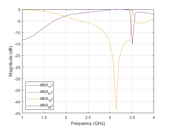
It is observed from the plot that its general trend is similar to that of w/o a shield except there is a box resonance around 3.5 GHz.