Basic Operations with RF Objects

This example shows how to read, analyze, and de-embed RF data from a Touchstone data file.

Video Walkthrough

For a walkthrough of the example, play the video.

Read and Analyze RF Data from Touchstone Data File

In this example, you create an sparameters object by reading the S-Parameters of a two-port passive network stored in the Touchstone format data file, passive.s2p.

Read S-Parameter data from a data file. Use RF Toolbox™ sparameters command to read the Touchstone data file, passive.s2p. This file contains 50-ohm S-Parameters at frequencies ranging from 315 kHz to 6 GHz. This operation creates an sparameters object, S_50, and stores data from the file in the object's properties.

S_50 = sparameters('passive.s2p');

Use sparameters to convert the 50-ohm S-Parameters in the sparameters object, to 75-ohm S-Parameters and save them in the variable S_75. You can easily convert between parameters, for example, for Y-Parameters from the sparameters object use yparameters and save them in the variable Y.

Znew = 75;
S_75 = sparameters(S_50, Znew);
Y    = yparameters(S_75);

Plot the S11 parameters. Use the smithplot command to plot the 75-ohm S11 parameters on a Smith® Chart:

smithplot(S_75,1,1)

View the 75-ohm S-Parameters and Y-Parameters at 6 GHz. Type the following set of commands at the MATLAB® prompt to display the 2-port 75-ohm S-Parameter values and the 2-port Y-Parameter values at 6 GHz.

freq    = S_50.Frequencies;
f       = freq(end)

f = 
6.0000e+09

s_6GHz  = S_75.Parameters(:,:,end)

s_6GHz = 2×2 complex

  -0.0764 - 0.5401i   0.6087 - 0.3018i
   0.6094 - 0.3020i  -0.1211 - 0.5223i

y_6GHz  = Y.Parameters(:,:,end)

y_6GHz = 2×2 complex

   0.0210 + 0.0252i  -0.0215 - 0.0184i
  -0.0215 - 0.0185i   0.0224 + 0.0266i

For more information, see the sparameters, yparameters, smithplot reference pages.

De-Embed S-Parameters

The Touchstone data file samplebjt2.s2p contains S-Parameter data collected from a bipolar transistor in a test fixture. The input of the fixture has a bond wire connected to a bond pad. The output of the fixture has a bond pad connected to a bond wire.

The configuration of the bipolar transistor, which is the device under test (DUT), and the fixture is shown in the following figure.

In this example, you remove the effects of the fixture and extract the S-parameters of the DUT.

Create RF circuit objects

Create a sparameters object for the measured S-Parameters by reading the Touchstone data file samplebjt2.s2p. Then, create two more circuit objects, one each for the input pad and output pad.

measured_data = sparameters('samplebjt2.s2p');

L_left      = inductor(1e-9);
C_left      = capacitor(100e-15);
input_pad   = circuit('inputpad');
add(input_pad,[1 2],L_left)
add(input_pad,[2 0],C_left)
setports(input_pad,[1 0],[2 0])

L_right     = inductor(1e-9);
C_right     = capacitor(100e-15);
output_pad  = circuit('outputpad');
add(output_pad,[3 0],C_right)
add(output_pad,[3 4],L_right)
setports(output_pad,[3 0],[4 0])

Analyze the input pad and output pad circuit objects. Analyze the circuit objects at the frequencies at which the S-Parameters are measured.

freq                = measured_data.Frequencies;
input_pad_sparams   = sparameters(input_pad,freq);
output_pad_sparams  = sparameters(output_pad,freq);

De-embed the S-parameters.

Extract the S-Parameters of the DUT from the measured S-Parameters by removing the effects of the input and output pads.

de_embedded_sparams = deembedsparams(measured_data,...
                      input_pad_sparams, output_pad_sparams);                  

Plot the measured and de-embedded S11 parameters. Type the following set of commands at the MATLAB® prompt to plot both the measured and the de-embedded S11 parameters on a Z Smith® Chart:

figure;
smithplot(measured_data,1,1);
hold on
h               = smithplot(de_embedded_sparams,1,1);
h.LineStyle     = {'-';'--'};
h.ColorOrder    = [1 0 0;0 0 1];
h.LegendLabels  = {'Measured S11', 'De-embedded S11'};

Plot the measured and de-embedded S22 parameters. Type the following set of commands at the MATLAB® prompt to plot the measured and the de-embedded S22 parameters on a Z Smith® Chart:

figure;
smithplot(measured_data,2,2);
hold on
h               = smithplot(de_embedded_sparams,2,2);
h.LineStyle     = {'-';':'};
h.ColorOrder    = [1 0 0;0 0 1];
h.LegendLabels  = {'Measured S22', 'De-embedded S22'};

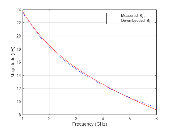
Plot the measured and de-embedded S21 parameters. Type the following set of commands at the MATLAB® prompt to plot the measured and the de-embedded S21 parameters, in decibels, on an X-Y plane:

figure
rfplot(measured_data,2,1,'db','r');
hold on
rfplot(de_embedded_sparams,2,1,'db',':b');
legend('Measured S_{21}', 'De-embedded S_{21}');

Related Topics

• RF Data Objects
• RF Circuit Objects
• RF Model Objects
• RF Network Parameter Objects