Characterize High-Frequency Data and Interconnects Using IEEE P370 Standard

Open Live Script

This example shows you how to use the IEEE P370 source code, its associated data files, and RF Toolbox™ functions to implement the following recommended practices for de-embedding the effect of fixtures when measuring a device under test (DUT).

S-parameters quality check: Perform quality checks on the S-parameters of the measured data.
Self de-embedding of 2X-Thru: Verify that the behavior of the self-de-embedded fixtures is transparent.
Compare the TDR of the fixture model to the FIX-DUT-FIX: Verify the assumption that the fixture model is identical to the fixture attached to the DUT.
Determine the similarity of S-parameters: Qualify and quantify the accuracy of the de-embedded DUT against the expected DUT.

For more information on the standard practices, see [1].

Introduction

De-embedding is the mathematical process of removing the unwanted effects of test fixtures that connect test equipment to the DUT in a measurement setup. De-embedding characterizes the effects of fixtures and uses the calculated calibration data to compensate for undesired distortions.

This example uses the following abbreviations:

2X-Thru: Connected replicas of the left and right fixtures, used for characterizing the effects of the fixtures
FIX-DUT-FIX: Composite structure of the test fixtures and the DUT during measurement

Setup

RF Toolbox ships IEEE P370 source files. Therefore, copy the contents from the +ieee370 package into a new folder in the MATLAB® working directory. Measured data files are included with this example and do not need to be copied.

ieee370Src = fullfile(matlabroot,"toolbox","rf","thirdparty","+ieee370");
ieee370Dir = fullfile(pwd,"ieee370");
copyfile(ieee370Src,ieee370Dir,"f")
addpath(ieee370Dir)

Extract the S-parameters of the 2x-Thru for de-embedding.

sFIX = sparameters("case_01_2xThru.s2p");
sdataFIX = sFIX.Parameters;
freqFIX  = sFIX.Frequencies;
nptsFIX = length(freqFIX);
portNumFIX = size(sdataFIX,1);

Extract the S-parameters of the FIX-DUT-FIX for de-embedding.

sFDF = sparameters("case_01_F-DUT1-F.s2p");
sdataFDF = sFDF.Parameters;
freqFDF = sFDF.Frequencies;
nptsFDF = length(freqFDF);
portNumFDF = size(sdataFDF,1);

Define the S-parameters of the DUT, which you use as a reference baseline to quantify the accuracy of the calculated DUT at the end of this example.

sDUT = sparameters("case_01_DUT1.s2p");
sdataDUT = sDUT.Parameters;
freqDUT = sDUT.Frequencies;

Suppress Warnings

The third-party IEEE P370 source files issue warnings. Suppress the warnings for the sake of keeping this example simple.

warnStruct = warning("off","MATLAB:colon:operandsNotRealScalar");
origWarnStatus = warnStruct.state;

S-Parameters Quality Check

Quantify the causality, reciprocity, and passivity of the 2X-Thru and FIX-DUT-FIX S-parameters to gauge the quality of the measurement. Perform this quality check using the frequency domain and time domain functions provided by IEEE P370.

Use IEEE P370 Frequency Domain Function

To get the causality, reciprocity, and passivity metrics of the S-parameters, call the function ieee370QualityCheckFrequencyDomain, which internally calls the IEEE P370 source function qualityCheckFrequencyDomain.

First, call the function on the measured 2X-Thru data.

[causalityMetricFIX_FD,reciprocityMetricFIX_FD,passivityMetricFIX_FD] =  ...
    ieee370QualityCheckFrequencyDomain(sdataFIX,nptsFIX,portNumFIX);

Next, call the function on the measured FIX-DUT-FIX data.

[causalityMetricFDF_FD,reciprocityMetricFDF_FD,passivityMetricFDF_FD] =  ...
    ieee370QualityCheckFrequencyDomain(sdataFDF,nptsFDF,portNumFDF);

Now, verify that the values of the metric indicate that the measured data pass the quality check. If the measurements fail, you must measure the structures again after recalibrating the measurement setup.

structure = ["2X-Thru" "FIX-DUT-FIX"];
for idx = 1:numel(structure)
    currStructure = structure(idx);
    switch currStructure
        case "2X-Thru"
            caus = causalityMetricFIX_FD;
            reci = reciprocityMetricFIX_FD;
            pass = passivityMetricFIX_FD;
        case "FIX-DUT-FIX"
            caus = causalityMetricFDF_FD;
            reci = reciprocityMetricFDF_FD;
            pass = passivityMetricFDF_FD;
    end

    reportCausality_FD(caus,currStructure)
    reportReciprocity_FD(reci,currStructure)
    reportPassivity_FD(pass,currStructure)
end

Causality for 2X-Thru is good (Frequency domain check).

Reciprocity for 2X-Thru is good (Frequency domain check).

Passivity for 2X-Thru is good (Frequency domain check).

Causality for FIX-DUT-FIX is good (Frequency domain check).

Reciprocity for FIX-DUT-FIX is good (Frequency domain check).

Passivity for FIX-DUT-FIX is good (Frequency domain check).

Use IEEE P370 Time Domain Function

Call the IEEE P370 qualityCheck function to perform the S-parameters check using a time domain method that constructs new S-parameters by enforcing passivity, causality, and reciprocity on the original data.

Set up variables to be used by qualityCheck.

portNum = 2;
dataRate = 2; % gbps
risePer = 0.1; % fractional rise time of UI
samplePerUI = 36;
pulseShape = 1; % 1 is Gaussian; 2 is rectangular with Butterworth filter; 3 is rectangular with Gaussian filter
extrapolationMethod = 2; % 1 is constant extrapolation; 2 is zero padding; 3 is repeating

Now, call qualityCheck on the 2X-Thru data, which produces plots that display the time response of the original and the constructed S-parameters. Ideally, the time responses of the original and constructed S-parameters must be identical, as the quality metric is based on quantifying the difference between the two. In the following plots, the results are visually similar, indicating that the data is most likely of good quality.

[causalityMetricFIX_TD,reciprocityMetricFIX_TD,passivityMetricFIX_TD] = ...
        qualityCheck(freqFIX,sdataFIX,portNum, ...
        dataRate,samplePerUI,risePer, ...
        pulseShape,extrapolationMethod, ...
        1);

causality_time_domain_difference_mv = 2×2

    0.0002    0.0036
    0.0036    0.0002

passivity_time_domain_difference_mv = 2×2
10^-15 ×

    0.2320    0.6724
    0.6678    0.4022

Next, call qualityCheck function on the FIX-DUT-FIX data. Once again, observe that the time responses of the original and constructed S-parameters are similar, indicating that the data is most likely of high quality.

[causalityMetricFDF_TD,reciprocityMetricFDF_TD,passivityMetricFDF_TD] = ...
        qualityCheck(freqFDF,sdataFDF,portNum, ...
        dataRate,samplePerUI,risePer, ...
        pulseShape,extrapolationMethod, ...
        5);

causality_time_domain_difference_mv = 2×2

    0.0002    0.0043
    0.0043    0.0002

passivity_time_domain_difference_mv = 2×2
10^-15 ×

    0.2048    0.6880
    0.5177    0.3136

Although the data seems to be of good quality based on visual inspection of the plots, quantitatively verify that the error is within the ranges suggested by IEEE P370.

for idx = 1:numel(structure)
    currStructure = structure(idx);
    switch currStructure
        case "2X-Thru"
            caus = causalityMetricFIX_TD;
            reci = reciprocityMetricFIX_TD;
            pass = passivityMetricFIX_TD;
        case "FIX-DUT-FIX"
            caus = causalityMetricFDF_TD;
            reci = reciprocityMetricFDF_TD;
            pass = passivityMetricFDF_TD;
    end

    reportCausality_TD(caus,currStructure)
    reportReciprocity_TD(reci,currStructure)
    reportPassivity_TD(pass,currStructure)
end

Causality for 2X-Thru is good (Time domain check).

Reciprocity for 2X-Thru is good (Time domain check).

Passivity for 2X-Thru is good (Time domain check).

Causality for FIX-DUT-FIX is good (Time domain check).

Reciprocity for FIX-DUT-FIX is good (Time domain check).

Passivity for FIX-DUT-FIX is good (Time domain check).

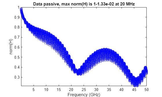
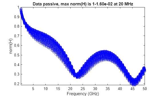
Cross-Validate with RF Toolbox

Cross-validate with RF Toolbox functions iscausal, ispassive, and passivity that the S-parameters are causal and passive. The plots from the passivity function illustrate that the data is less than unity, indicating passivity.

for idx = 1:numel(structure)
    currStructure = structure(idx);
    switch currStructure
        case "2X-Thru"
            S = sFIX;
        case "FIX-DUT-FIX"
            S = sFDF;
    end

    if iscausal(S)
        disp(currStructure + " is causal according to iscausal function.")
    else
        disp(currStructure + "is not causal according to iscausal function.")
    end

    if ispassive(S)
        disp(currStructure + " is passive according to ispassive function.")
    else
        disp(currStructure + "is not passive according to ispassive function.")
    end
    figure
    passivity(S)
end

2X-Thru is causal according to iscausal function.

2X-Thru is passive according to ispassive function.

FIX-DUT-FIX is causal according to iscausal function.

FIX-DUT-FIX is passive according to ispassive function.

Self De-embedding of 2X-Thru

To verify the assumptions of the de-embedding algorithm are appropriate for the fixtures, de-embed the 2X-Thru from itself to check that the result is an electrically transparent interconnect [1].

Self De-embed

Call the IEEEP3702xThru function to extract the error boxes representing the left and right halves of a 2-port 2X-Thru. You can also use the IEEE function IEEEP370mmZc2xthru to extract error boxes from mixed mode S-parameters.

[sFIX1,sFIX2] = IEEEP3702xThru(sFIX);

Calculate the de-embeded 2X-Thru.

sFIX_deembed = deembedsparams(sFIX,sFIX1,sFIX2);

Check De-embeded 2X-Thru

Plot the magnitude and phase of the self-de-embedded 2X-Thru to observe that the following criteria are met:

Absolute value of the magnitude of residual insertion loss is < 0.1 dB.
Phase of self-de-embedded 2X-Thru is < 1 deg.

sFIX21 = squeeze(sFIX_deembed.Parameters(2,1,:));

figure
hAx = subplot(2,1,1);
plot(hAx,freqFIX,db(sFIX21));
xlabel(hAx,"Frequency (Hz)"),ylabel(hAx,"Magnitude (dB)")
legend("dB (S21)")
title(hAx,"S21 self de-embedding amplitude")

hAx = subplot(2,1,2);
plot(hAx,freqFIX,angle(sFIX21));
xlabel(hAx,"Frequency (Hz)"),ylabel(hAx,"Angle (degrees)")
legend("deg (S21)")
title(hAx,"S21 self de-embedding angle")

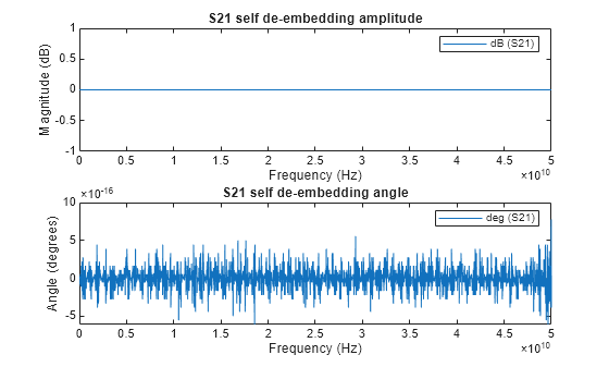
These plots show that the magnitude is 0 and the angle is less than 1e-16, suggesting that the self-de-embedding is successful.

Compare TDR of Fixture Model and FIX-DUT-FIX

Verify assumption that the fixture model is identical to the fixture attached to the DUT by comparing their time-domain reflectometer (TDR) responses.

Calculate TDR

Visualize the TDR responses of the 2X-Thru and the FIX-DUT-FIX by calling the IEEE P370 function compare_s2x_fdf_tdr.

compare_s2x_fdf_tdr(sFIX,sFDF)

Use the TDR response calculated and displayed in the previous steps to validate the behavior of the fixtures on the 2X-Thru and FIX-DUT-FIX. To source the data from the plots, use the helper function getTdrData.

[zdataFIX,zdataFDF,timeFIX,timeFDF,hFigs] = getTdrData;

Compare TDRs

Inspect the TDR plots to set the start of the fixture to the time of the midpoint of the 2X-Thru. The start and midpoint times for port 1 and port 2 are identical, indicating that you can use the same computations for both ports.

assert(isequal(timeFIX,timeFDF))
t = timeFIX;

tStart = 0.07;
tEnd = 0.56;
[~,idxStart] = min(abs(t-tStart));
[~,idxEnd] = min(abs(t-tEnd));

zdataFIX1 = zdataFIX(:,1);zdataFIX2 = zdataFIX(:,2);
zdataFDF1 = zdataFDF(:,1);zdataFDF2 = zdataFDF(:,1);

hFig = hFigs(1); hAx = hFig.CurrentAxes;
text(hAx,tStart,zdataFIX1(idxStart),"\leftarrow START","FontWeight","bold")
text(hAx,tEnd,zdataFIX1(idxEnd),sprintf("MIDPOINT\n") + "\downarrow","FontWeight","bold","VerticalAlignment","bottom")

hFig = hFigs(2); hAx = hFig.CurrentAxes;
text(hAx,tStart,zdataFIX2(idxStart),"\leftarrow START","FontWeight","bold")
text(hAx,tEnd,zdataFIX2(idxEnd),sprintf("MIDPOINT\n") + "\downarrow","FontWeight","bold","VerticalAlignment","bottom")

Measure the point-wise difference between the 2X-Thru impedance and the FIX-DUT-FIX impedance from the start to the midpoint.

absDiff1 = abs(zdataFIX1(idxStart:idxEnd)-zdataFDF1(idxStart:idxEnd));
absDiff2 = abs(zdataFIX2(idxStart:idxEnd)-zdataFDF2(idxStart:idxEnd));

Assuming the most stringent requirements, verify that the difference from the reference impedance is within ±2.5%.

assert(sFIX.Impedance==sFDF.Impedance)
Z = sFIX.Impedance;

assert(max(absDiff1./Z) < 0.025)
assert(max(absDiff2./Z) < 0.025)

Determine Similarity of Expected and De-embedded S-parameters of DUT

De-embed the DUT from the fixtures. Compare the de-embedded result against the expected original DUT.

sDUT_deembed = deembedsparams(sFDF,sFIX1,sFIX2);
sdataDUT_deembed = sDUT_deembed.Parameters;

Perform Qualitative Measure of Accuracy

Visually compare the de-embedded DUT against the original DUT. Ideally, the de-embedded results and the original results must be identical.

figure
plotComparisonDUT(sdataDUT_deembed,sdataDUT,freqFDF,freqDUT)
sgtitle("Qualitative Results (IEEE P370)")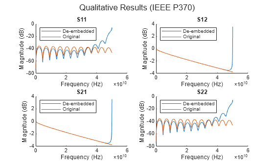

Perform Quantitative Measure of Accuracy

Calculate the absolute error between the de-embedded DUT and the original DUT and report it in dB.

figure
plotErrorDUT(sdataDUT_deembed,sdataDUT,freqFDF)
sgtitle("Quantitative Results (IEEE P370)")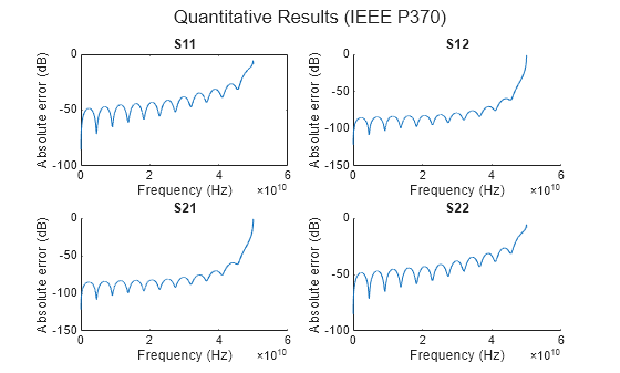

Improved Algorithm for Extracting Error Boxes

The de-embedded results from the Determine the similarity of S-parameters section begin to deviate from the expected results at frequencies around 40 GHz, resulting in errors worse than -40 dB. This deviation is an artifact caused by ripples originating from the sinc due to windowing performed during the extraction of the left and right fixtures. The effect is accentuated at higher frequencies due to the boundary discontinuity resulting from the circular nature of the DFT [2].

You can overcome these inherent limitations of windowing and the DFT by utilizing a continuous time technique [3]. By representing the signal as a Laplace domain partial fraction, the time gating operations are not reliant on the periodic assumptions of the DFT and thus avoid the boundary discontinuity. In fact, because the gate width is infinite in this context, you can completely eliminate the ripples, as the windowing by modeling a Heaviside step function.

Once again implement steps in the Self De-embed section by using the enhanced version of the IEEE P370 function IEEEP3702xThru_ModifiedTimeGate to conduct de-embedding with higher accuracy.

[sFIX1_improved,sFIX2_improved] = IEEEP3702xThru_ModifiedTimeGate(sFIX);
sFIX_deembed_improved = deembedsparams(sFIX,sFIX1_improved,sFIX2_improved);

sDUT_deembed_improved = deembedsparams(sFDF,sFIX1_improved,sFIX2_improved);
sdataDUT_deembed_improved = sDUT_deembed_improved.Parameters;

Visually compare the de-embedded DUT against the original DUT. The actual de-embedded results are substantially closer to the expected original data, especially at higher frequencies.

figure
plotComparisonDUT(sdataDUT_deembed_improved,sdataDUT,freqFDF,freqDUT,"southwest")
sgtitle("Qualitative Results (IEEE P370 Modified)")

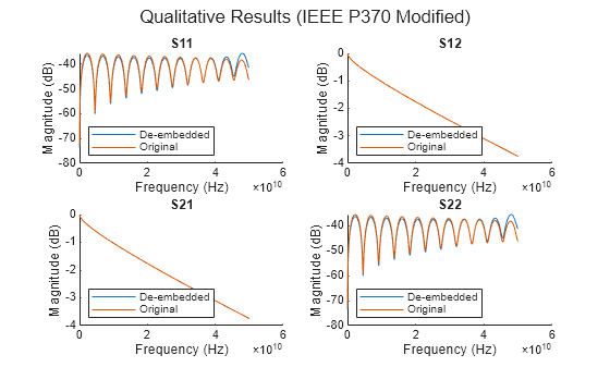
Plot the error. Observe that the highest error is below -40 dB, which is better than the maximum error of the unmodified IEEE P370 algorithm.

figure
plotErrorDUT(sdataDUT_deembed_improved,sdataDUT,freqFDF)
sgtitle("Quantitative Results (IEEE P370 Modified)")

Clean up

Clean up the warnings that you suppressed earlier in the example.

warnStruct = warning(origWarnStatus,'MATLAB:colon:operandsNotRealScalar');

References

[1] "IEEE Standard for Electrical Characterization of Printed Circuit Board and Related Interconnects at Frequencies up to 50 GHz". IEEE Std 370-2020, vol., no., pp.1-147. 8 Jan. 2021. doi: 10.1109/IEEESTD.2021.9316329.

[2] Oppenheim, Alan V., Ronald W. Schafer, and John R. Buck. Discrete-Time Signal Processing. 2nd ed. Upper Saddle River, N.J: Prentice Hall, 1999.

[3] Reeves T. "Time Domain Gating of Microwave Component Responses Using Analog Techniques". EDICON, 2016.