Assessing Performance with the Tracker Operating Characteristic
This example shows how to assess the:
Probability of target track: The target track detection probability for a single target with and without the presence of false alarms
Probability of false track: False track probability due to false alarms in the neighborhood of a single target
This example discusses different methods to perform these calculations with varying levels of fidelity and computation time.
In the assessment of tracker performance, four types of probabilities are often calculated:
Probability of a single target track in the absence of false alarms (probability of false alarm )
Probability of a single false track in the absence of targets (probability of detection )
Probability of a single target track in the presence of false alarms
Probability of a single false track in the presence of targets
This example first calculates the probability of single target track in the absence of false alarms using the Bernoulli sum. Then, it discusses the common gate history (CGH) algorithm that can be used to calculate all 4 types of probabilities and introduces the concept of the tracker operating characteristic (TOC), which is similar in form to the receiver operating characteristic (ROC). The CGH algorithm provides an estimate of system capacity and offers a means to assess end-to-end system performance. Lastly, the example presents the CGH algorithm as applied to an automotive radar design scenario and assists users in the selection of:
Required target signal-to-noise ratio (SNR)
Number of false tracks
Tracker confirmation threshold
Calculate Single Target Track Probability in the Absence of False Alarms
Bernoulli Sum
The Bernoulli sum allows for quick and easy performance analysis in the case of a single target in the absence of false alarms. The track detection probability can be defined in terms of the receiver detection probability for a window period defined as
,
where T is the basic sampling period and N represents the number of opportunities for a detection.
For a confirmation threshold logic of M-of-N, the target track probability is defined as
,
where
.
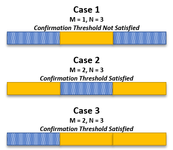
The confirmation threshold logic denoted as M-of-N or M/N is a one-stage logic where a track must associate to a detection, also known as a hit, at least M times out of N consecutive looks. For example, consider a 2-of-3 logic. In the following figure, the solid yellow represents a hit, which can be from either a target or a false alarm. The patterned blue blocks represent misses. The cases represented below are not intended to be exhaustive, but the figure indicates cases 2 and 3 satisfy the threshold, but case 1 does not.
Investigate the probability of target track versus probability of detection for a confirmation threshold of 2/3 using the Bernoulli sum method. Perform the Bernoulli sum calculation, assuming that one hit is required to initialize a track.
% Define probabilities for analysis
Pd = linspace(0,1,100).';

% Define confirmation threshold M/N
M = 2; % Number of hits
N = 3; % Number of observations or opportunities

% Calculate Bernoulli sum, assuming 1 hit is required to initialize a track
tic
PdtBernoulli = helperBernoulliSum(Pd,M,N);
elapsedTime = toc;
helperUpdate('Bernoulli',elapsedTime);
Bernoulli calculation completed. Total computation time is 0.0155 seconds.
% Plot the probability of detection versus the probability of target track
hAxes = helperPlot(Pd,PdtBernoulli,'M/N = 2/3','P_D','P_{DT}', ...
    sprintf('Bernoulli Sum\nProbability of Target Track in the Absence of False Alarms'));

% Set desired probability of target track
yline(hAxes,0.9,'--','LineWidth',2,'DisplayName','Desired P_{DT}');
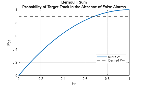
Assuming a required probability of target track of 0.9, the plot above indicates that a detection probability of about 0.7 is necessary.
Calculate Probabilities for Targets in Clutter
The values obtained from a Bernoulli sum calculation are useful in quick analyses, but are not generally representative of real tracking environments, where target tracks are affected by the presence of false alarms. Consider the scenario where a target is operating in the presence of clutter.
Assuming that false alarms occur on a per-look per-cell basis, the probability of false alarms in a tracking gate depend upon the number of cells in the gate. Assume three types of events:
Miss: No detection
Hit: False alarm
Hit: Target detection
The number of cells in a gate depends upon the history of events and the order in which events occur. These factors dictate the gate growth sequence of the tracker.
The Bernoulli sum method assumes that there are no false alarms and that the order of detections does not matter. Thus, when you use the Bernoulli sum in the target in clutter scenario, it produces overly optimistic results.
One approach for analyzing such scenarios is to evaluate every possible track sequence and determine which sequences satisfy the confirmation threshold logic. This brute-force approach of building the Markov chain is generally too computationally intensive.
Another approach is to utilize a Monte Carlo-type analysis. Rather than generating the full Markov chain, a Monte Carlo simulation manually generates random sequences of N events. The confirmation threshold is applied to each sequence, and statistics are aggregated. The Monte Carlo method is based upon the law of large numbers, so performance improves as the number of iterations increases. Monte Carlo analysis lends itself well to parallelization, but in the case of small probabilities of false alarm, the number of iterations can become untenable. Thus, alternative methods to quickly calculate track probability measures are needed.
The Common Gate History Algorithm
The common gate history (CGH) algorithm greatly reduces computation times and memory requirements. The algorithm avoids the need for manual generation of sequences, as in the case of Monte Carlo analysis, which can be costly for low-probability events.
The algorithm begins by making the assumption that there are three types of tracks, which can contain:
Detections from targets
Detections from targets and false alarms
Detections from false alarms only
A target track is defined as any track that contains at least one target detection and satisfies the M/N confirmation threshold. Thus, track types 1 and 2 are considered to be target tracks, whereas 3 is considered to be a false track.
Given the previously defined track types and with a confirmation threshold logic M/N, a unique track state is defined as
,
where is the number of time steps since the last detection (target or false alarm), is the number of time steps since the last target detection, and is the total count of detections (targets or false alarms). As the algorithm proceeds, the track state vector evolves according to a Markov chain.
The algorithm assumes that a track can be started given only two types of events:
Target detection
False alarm
Once a track is initiated, the following four types of events continue a track:
No detection
Target detection
False alarm
Target detection and false alarm
The track probability at look m is multiplied by the probability of the event that continues the track at look . The tracks are then lumped by adding the track probabilities of the track files with a common gate history vector. This lumping keeps the number of track states in the Markov chain within reasonable limits.
The assumptions of the CGH algorithm are as follows:
The probability of more than one false alarm in a gate is low, which is true when the probability of false alarm is low ( or less)
The location of a target in a gate has a uniform spatial distribution
A track splitting algorithm is used
The CGH algorithm can be used to calculate all four probability types:
Probability of a single target track in the absence of false alarms
Probability of a single false track in the absence of targets
Probability of a single target track in the presence of false alarms
Probability of a single false track in the presence of targets
The probability of target track and the probability of false track form the basis of the tracker operating characteristic (TOC). The TOC compliments the receiver operating characteristic (ROC), which is commonly used in the analysis and performance prediction of receivers. Combining the ROC and the TOC provides an end-to-end system analysis tool.
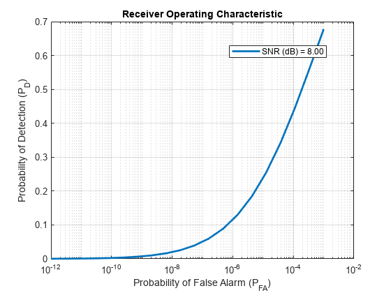
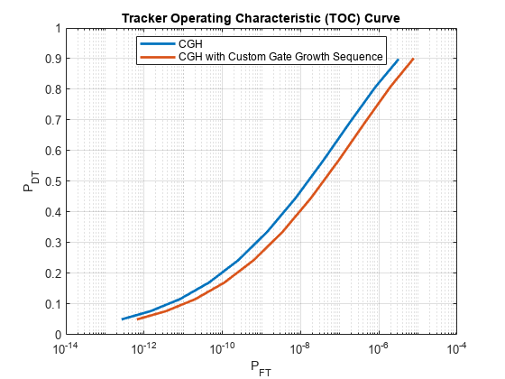
Calculate and plot the TOC using ROC curves from rocsnr as inputs. Assume a signal-to-noise ratio (SNR) of 8 dB. Continue to use the 2/3 confirmation threshold logic as in the Bernoulli sum example. Use the toccgh built-in tracker.
% Receiver operating characteristic (ROC)
snrdB = 8; % SNR (dB)
[Pd,Pfa] = rocsnr(snrdB,'MaxPfa',1e-3,'MinPfa',1e-12,'NumPoints',20);

% Plot ROC
helperPlotLog(Pfa,Pd,snrdB, ...
    'Probability of False Alarm (P_{FA})', ...
    'Probability of Detection (P_D)', ...
    'Receiver Operating Characteristic');
% CGH algorithm
tic
[PdtCGH,PftCGH] = toccgh(Pd,Pfa,'ConfirmationThreshold',[M N]);
elapsedTime = toc;
helperUpdate('Common Gate History',elapsedTime);
Common Gate History calculation completed. Total computation time is 0.6090 seconds.
% Plot CGH results
hAxes = helperPlotLog(PftCGH,PdtCGH,'CGH','P_{FT}','P_{DT}', ...
    'Tracker Operating Characteristic (TOC) Curve');
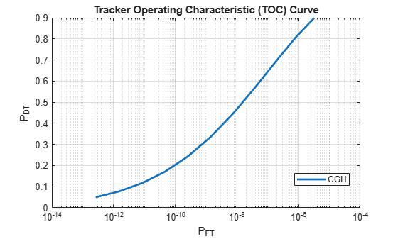
The CGH algorithm permits the assessment of tracker performance similar to a Monte Carlo analysis but with acceptable computation times despite low-probability events. The CGH algorithm thus permits high-level investigation and selection of options prior to more intensive, detailed simulations.
Using CGH with Custom Trackers
Consider a tracker for an automotive application. Define a custom, one-dimensional, nearly constant velocity (NCV) tracker using trackingKF. Assume that the update rate is 1 second. Assume that the state transition matrix is of the form
and the process noise is of the form
,
where is a tuning factor defined as
.
The input is the maximum target acceleration expected. Assume that a maximum acceleration of 4 m/s is expected for vehicles.
% Define the state transition matrix
dt = 1; % Update rate (sec)
A = [1 dt; 0 1];

% Define the process noise
Q = [dt^4/4 dt^3/2; dt^3/2 dt^2];

% Tune the process noise
amax = 4; % Maximum target acceleration (m/s^2)
q = amax^2*dt;

% Update the process noise
Q = Q.*q;

% Initialize the Kalman filter
trkfilt = trackingKF('MotionModel','Custom', ...
    'StateCovariance', [0 0; 0 0], ...
    'StateTransitionModel',A, ...
    'ProcessNoise',Q, ...
    'MeasurementNoise',0, ...
    'MeasurementModel',[1 0]);
An error ellipse is used to model track uncertainty. From this uncertainty ellipse, the gate growth sequence can be calculated.
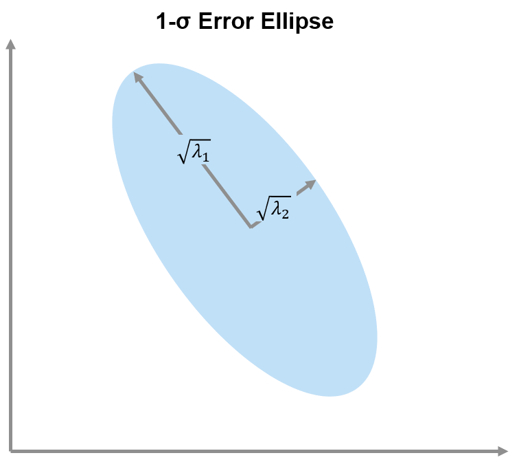
The 1- values of the error ellipse are calculated as the square root of the eigenvalues of the predicted state covariance :
.
The area of the error ellipse is then calculated as
.
The area of the bins is calculated as
.
Finally, the gate size in bins is
.
The gate size is thus dependent upon the tracker, the event sequence, and the resolution of the bins. Calculate the gate growth sequence, assuming a confirmation threshold N equal to 3. Assume the range and range rate resolutions for the automotive radar are equal to 1 meter and 1 m/s, respectively.
% Calculate gate growth sequence
res = [1, 1]; % Bin resolutions [range (m), range-rate (m/s)]
gs = helperCalculateGateSize(N,trkfilt,res)
gs = 1×3

     1    51   124
% CGH algorithm
tic
[PdtCGHcustom,PftCGHcustom] = toccgh(Pd,Pfa,'ConfirmationThreshold',[M N],'GateGrowthSequence',gs);
elapsedTime = toc;
helperUpdate('Common Gate History',elapsedTime);
Common Gate History calculation completed. Total computation time is 0.0406 seconds.
% Add plot to previous plot
helperAddPlotLog(hAxes,PftCGHcustom,PdtCGHcustom,'CGH with Custom Gate Growth Sequence');
Tracker Performance Assessment for an Automotive Radar System
Probability of False Alarm and Probability of Target Track Requirements
By using the ROC and TOC in conjunction, a system analyst can select a detector's operation point that satisfies the overall system requirements. Consider an automotive radar case. Due to the nature of the application, it is desired that false alarms remain very low probability events. Additionally, the probability of target track should be high for safety purposes. Consider the following two requirements.
Requirement 1 Probability of false alarm must be less than
Requirement 2 Probability of target track must be equal to 0.9 or above
Calculate the ROC curves for SNRs equal to 6, 8, 10, and 12 dB.
% Calculate ROC curves
snrdB = [6 8 10 12]; % SNR (dB)
[Pd,Pfa] = rocsnr(snrdB,'MaxPfa',1e-3,'MinPfa',1e-10,'NumPoints',10);
Use the calculated ROC curves as inputs to the toccgh function to generate the associated TOC curves. Use the same confirmation threshold and gate growth sequence previously generated.
% Generate TOC curves
tic
toccgh(Pd,Pfa,'ConfirmationThreshold',[M N],'GateGrowthSequence',gs);
elapsedTime = toc;
helperUpdate('Common Gate History',elapsedTime);
Common Gate History calculation completed. Total computation time is 0.4267 seconds.
% Requirement 1: Probability of false alarms must be less than 1e-6
hAxesROC = subplot(2,1,1);
xlim([1e-10 1e-2])
ylim([0 1])
reqPfa = 1e-6;
helperColorZonesReqPfa(hAxesROC,reqPfa)
legend(hAxesROC,'Location','eastoutside')

% Requirement 2: Probability of target track must be equal to 0.9 or above
hAxesTOC = subplot(2,1,2);
xlim([1e-14 1e-4])
ylim([0 1])
reqPdt = 0.9;
helperColorZonesReqPdt(hAxesTOC,reqPdt)

Requirement 1 indicates that only points 1 through 6 on the ROC curves can be included for further analysis since they satisfy a probability lower than . Points 7 through 10 do not meet this requirement.
Regarding requirement 2, the ROC curve corresponding to 6 dB SNR does not meet the second requirement at any point. The only curves to continue considering are the 8, 10, and 12 dB curves. Requirement 2 is met only for point 10 on the 8 dB curve, points 9 and 10 on the 10 dB curve, and points 5 through 10 on the 12 dB curve.
Combining requirements 1 and 2, only two analysis points satisfy both requirements points 5 and 6 on the 12 dB curve. Point 5 corresponds to a probability of target track of 0.90 and a probability of false track of , which corresponds to a probability of detection of 0.68 and a probability of false alarm of . Similarly, point 6 corresponds to a probability of target track of 0.96, probability of false track of , probability of detection of 0.80, and a probability of false alarm of . Select point 6, which represents a tradeoff of improved probability of target track at the expense of a slightly higher but reasonable probability of false track.
The CGH algorithm permits an estimation of the expected number of false tracks based on the number of targets anticipated in an environment and the number of cells in the radar data. The expected number of false tracks is calculated as
,
where is the probability of false track in the absence of targets, is the number of cells, is the probability of false track in the presence of targets, and is the number of targets.
Consider an environment where the number of targets is expected to be equal to 10 and the number of cells is equal to
% Calculate expected number of false tracks using toccgh
numCells = 1e5;         % Number of cells in radar data
numTargets = 10;        % Number of targets in scenario
selectedPd = Pd(6,4) ;  % Selected probability of detection
selectedPfa = Pfa(6);   % Selected probability of false alarm
[Pdt,Pft,Eft] = toccgh(selectedPd,selectedPfa, ...
    'ConfirmationThreshold',[M N],'GateGrowthSequence',gs, ...
    'NumCells',numCells,'NumTargets',10);

% Output results
helperPrintTrackProbabilities(Pdt,Pft,Eft);
Probability of Target Track in Presence of False Alarms = 0.9581
Probability of False Track in the Presence of Targets = 1.6410e-12
Expected Number of False Tracks = 5
Thus, based on the system parameters, you can expect about five false tracks.
Analysis of Confirmation Thresholds
Consider the same automotive radar design case but investigate the effect of confirmation thresholds 2/4, 3/4, and 4/4. Assume the following:
Requirement 1 Probability of false alarm must be less than
Requirement 2 Probability of target track must be equal to 0.9 or above
First, calculate the ROC curve using the rocpfa function.
% Calculate ROC curve assuming a probability of false alarm of 1e-6
Pfa = 1e-6;
numPoints = 20;
[Pd,snrdB] = rocpfa(Pfa,'NumPoints',numPoints,'MaxSNR',15);
Update the gate growth sequence due to the greater number of observations.
% Update the gate growth sequence
N = 4;
trkfilt = trackingKF('MotionModel','Custom', ...
    'StateCovariance', [0 0; 0 0], ...
    'StateTransitionModel',A, ...
    'ProcessNoise',Q, ...
    'MeasurementNoise',0, ...
    'MeasurementModel',[1 0]);
gs = helperCalculateGateSize(N,trkfilt,res)
gs = 1×4

     1    51   124   225
Calculate the TOC given the ROC curves as inputs and confirmation thresholds equal to 2/4, 3/4, and 4/4.
% Calculate TOC
cp = [2 4; 3 4; 4 4];
numCp = size(cp,1);
PdtMat = zeros(numPoints,numCp);
PftMat = zeros(numPoints,numCp);
EftMat = zeros(numPoints,numCp);
for ii = 1:numCp
    [PdtMat(:,ii),PftMat(:,ii),EftMat(:,ii)] = toccgh(Pd.',Pfa, ...
        'ConfirmationThreshold',cp(ii,:),'GateGrowthSequence',gs, ...
        'NumCells',numCells,'NumTargets',10);
end

% Plot ROC and TOC
reqPdt = 0.9;
helperPlotROCTOC(reqPdt,Pfa,Pd,snrdB,PdtMat,cp);
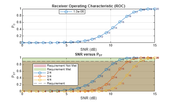
helperPrintReqValues(reqPdt,Pd,snrdB,PdtMat,EftMat,cp);
Confirmation Threshold            = 2/4
Required Probability of Detection = 0.55
Required SNR (dB)                 = 10.76
Expected Number of False Tracks   = 18

Confirmation Threshold            = 3/4
Required Probability of Detection = 0.81
Required SNR (dB)                 = 12.03
Expected Number of False Tracks   = 1

Confirmation Threshold            = 4/4
Required Probability of Detection = 0.97
Required SNR (dB)                 = 13.37
Expected Number of False Tracks   = 1
Reviewing the results, you can see that the more stringent the confirmation threshold, the higher the required SNR. However, the more stringent confirmation thresholds result in improved numbers of false tracks.
Summary
In the assessment of tracker performance, four types of probabilities are often calculated:
Probability of a single target track in the absence of false alarms
Probability of a single false track in the absence of targets
Probability of a single target track in the presence of false alarms
Probability of a single false track in the presence of targets
For the calculation of 1, Bernoulli sums can be used. However, to obtain the other probabilities, a different method must be employed. Monte Carlo analysis can be used for the computation of the latter three types of probabilities, but the computational resources and time required can become untenable, which is particularly true for events with low probability. The common gate history (CGH) algorithm can be used to calculate all four quantities and greatly reduces computational resources needed.
The CGH algorithm can be used to generate the tracker operating characteristic (TOC). The TOC compliments the receiver operating characteristic (ROC) and provides a means to assess overall system performance. The TOC and ROC curves can be used in a multitude of ways such as determining:
Required target signal-to-noise ratio (SNR)
Tracker confirmation threshold
Finally, the CGH algorithm permits the calculation of an expected number of false tracks, which offers insights into system capacity. The expected number of false tracks can be used to ascertain computational load and to assist with decisions related to hardware and processing.
References
Bar-Shalom, Y., et al. "From Receiver Operating Characteristic to System Operating Characteristic: Evaluation of a Track Formation System." IEEE Transactions on Automatic Control, vol. 35, no. 2, Feb. 1990, pp. 172-79. DOI.org (Crossref), doi:10.1109/9.45173.
Bar-Shalom, Yaakov, et al. Tracking and Data Fusion: A Handbook of Algorithms. YBS Publishing, 2011.
Helper Functions
function Pcnf = helperBernoulliSum(Pd,Mc,Nc)
% Calculate simple Bernoulli sum. Use the start TOC logic, which assumes
% that there is already one hit that initializes the track.

% Update M and N for probability of deletion
Nd = Nc - 1;      % Need one hit to start counting. Assume first hit initializes track.
Md = Nc - Mc + 1; % Need this many misses to delete

% Bernoulli sum. Probability of deletion calculation.
ii = Md:Nd;
C = arrayfun(@(k) nchoosek(Nd,k),ii);
P = (1 - Pd);
Pdel = sum(C.*P(:).^ii.*(1 - P(:)).^(Nd - ii),2);

% Probability of confirmation
Pcnf = 1 - Pdel;
end

function helperUpdate(calculationType,elapsedTime)
% Output elapsed time
fprintf('%s calculation completed. Total computation time is %.4f seconds.\n', ...
        calculationType,elapsedTime);
end

function varargout = helperPlot(x,y,displayName,xAxisName,yAxisName,titleName,varargin)
% Create a plot with logarithmic scaling on the x-axis

% Create a figure
figure('Name',titleName)
hAxes = gca;

% Plot data
plot(hAxes,x,y,'LineWidth',2,'DisplayName',displayName,varargin{:})
hold(hAxes,'on')
grid(hAxes,'on')

% Update axes
hAxes.Title.String = titleName;
hAxes.XLabel.String = xAxisName;
hAxes.YLabel.String = yAxisName;

% Make sure legend is on and in best location
legend(hAxes,'Location','Best')

% Set axes as optional output
if nargout == 1
    varargout{1} = hAxes;
end
end

function varargout = helperPlotLog(x,y,displayName,xAxisName,yAxisName,titleName,varargin)
% Create a plot with logarithmic scaling on the x-axis

% Create a figure
figure('Name',titleName)
hAxes = gca;

% Plot data
numCol = size(y,2);
for ii = 1:numCol
    idxX = min(ii,size(x,2));
    hLine = semilogx(hAxes,x(:,idxX),y(:,ii),'LineWidth',2,varargin{:});
    if ischar(displayName)
        hLine.DisplayName = displayName;
    else
        hLine.DisplayName = sprintf('SNR (dB) = %.2f',displayName(ii));
    end
    hold on
end
grid on

% Update axes
hAxes.Title.String = titleName;
hAxes.XLabel.String = xAxisName;
hAxes.YLabel.String = yAxisName;

% Make sure legend is on and in best location
legend(hAxes,'Location','Best')

% Set axes as optional output
if nargout == 1
    varargout{1} = hAxes;
end
end

function helperAddPlotLog(hAxes,x,y,displayName,varargin)
% Add an additional plot to the axes hAxes with logarithmic scaling on the
% x-axis

% Plot data
hold on
hLine = semilogx(hAxes,x,y,'LineWidth',2,varargin{:});
hLine.DisplayName = displayName;
end

function gs = helperCalculateGateSize(N,trkfilt,res)
% Calculate a gate growth sequence in bins

% Initialize tracker gate growth sequence
gs = zeros(1,N); % Gate growth sequence

% Calculate gate growth sequence by projecting state uncertainty using
% linear approximations.
areaBin = prod(res(:),1);
for n = 1:N
    [~,Ppred] = predict(trkfilt); % Predict

    % Calculate the products of the 1-sigma values
    E = eig(Ppred);
    E(E<0) = 0; % Remove negative values
    sigma1Prod = sqrt(prod(E(:),1));

    % Calculate error ellipse area
    areaErrorEllipse = pi*sigma1Prod; % Area of ellipse = pi*a*b

    % Translate to bins
    gs(n) = max(ceil(areaErrorEllipse/areaBin),1);
end
end

function helperColorZonesReqPfa(hAxes,req)
% Plot color zones for requirement type 1

% Vertical requirement line
xline(req,'--','DisplayName','Requirement',...
    'HitTest','off');

% Get axes limits
xlims = get(hAxes,'XLim');
ylims = get(hAxes,'YLim');

% Green box
pos = [xlims(1) ylims(1) req ylims(2)];
x = [pos(1) pos(1) pos(3) pos(3) pos(1)];
y = [pos(1) pos(4) pos(4) pos(1) pos(1)];
hP = patch(hAxes,x,y,[0.4660 0.6740 0.1880], ...
    'FaceAlpha',0.3,'EdgeColor','none','DisplayName','Requirement Met');
uistack(hP,'bottom');

% Red box
pos = [req ylims(1) xlims(2) ylims(2)];
x = [pos(1) pos(1) pos(3) pos(3) pos(1)];
y = [pos(1) pos(4) pos(4) pos(1) pos(1)];
hP = patch(hAxes,x,y,[0.6350 0.0780 0.1840], ...
    'FaceAlpha',0.3,'EdgeColor','none','DisplayName','Requirement Not Met',...
    'HitTest','off');
uistack(hP,'bottom');
end

function helperColorZonesReqPdt(hAxes,req)
% Plot color zones for requirement type 2

% Horizontal requirement line
yline(req,'--','DisplayName','Requirement',...
    'HitTest','off')

% Get axes limits
xlims = get(hAxes,'XLim');
ylims = get(hAxes,'YLim');

% Green box
pos = [xlims(1) req xlims(2) ylims(2)];
x = [pos(1) pos(1) pos(3) pos(3) pos(1)];
y = [pos(1) pos(4) pos(4) pos(1) pos(1)];
hP = patch(hAxes,x,y,[0.4660 0.6740 0.1880], ...
    'FaceAlpha',0.3,'EdgeColor','none','DisplayName','Requirement Met',...
    'HitTest','off');
uistack(hP,'bottom');

% Red box
pos = [xlims(1) req xlims(2) req];
x = [pos(1) pos(1) pos(3) pos(3) pos(1)];
y = [pos(1) pos(4) pos(4) pos(1) pos(1)];
hP = patch(hAxes,x,y,[0.6350 0.0780 0.1840], ...
    'FaceAlpha',0.3,'EdgeColor','none','DisplayName','Requirement Not Met',...
    'HitTest','off');
uistack(hP,'bottom');
end

function helperPrintTrackProbabilities(Pdt,Pft,Eft)
% Print out results

fprintf('Probability of Target Track in Presence of False Alarms = %.4f\n',Pdt)
fprintf('Probability of False Track in the Presence of Targets = %.4e\n',Pft)
fprintf('Expected Number of False Tracks = %d\n',Eft)
end

function helperPlotROCTOC(reqPdt,Pfa,Pd,snrdB,PdtMat,cp)
% Plot ROC/TOC

% Plot ROC curves
figure
hAxesROC = subplot(2,1,1);
plot(hAxesROC,snrdB,Pd,'-o')
title(hAxesROC,'Receiver Operating Characteristic (ROC)')
xlabel(hAxesROC,'SNR (dB)')
ylabel(hAxesROC,'P_D')
grid(hAxesROC,'on')
legend(hAxesROC,sprintf('%.1e',Pfa),'Location','Best')

% Plot SNR versus probability of target track
hAxesTOC = subplot(2,1,2);
numCp = size(cp,1);
for ii = 1:numCp
    plot(hAxesTOC,snrdB,PdtMat(:,ii),'-o', ...
        'DisplayName',sprintf('%d/%d',cp(ii,1),cp(ii,2)))
    hold(hAxesTOC,'on')
end
title(hAxesTOC,'SNR versus P_{DT}')
xlabel(hAxesTOC,'SNR (dB)')
ylabel(hAxesTOC,'P_{DT}')
grid(hAxesTOC,'on')
legend(hAxesTOC,'Location','Best')

% Label points
colorVec = get(hAxesROC,'ColorOrder');
numSnr = numel(snrdB);
textArray = arrayfun(@(x) sprintf('  %d',x),1:numSnr,'UniformOutput',false).';
xPosROC = snrdB;
colorFont = brighten(colorVec,-0.75);
numColors = size(colorVec,1);
idxC = mod(1:numCp,numColors); % Use only available default colors
idxC(idxC == 0) = numColors; % Do not let color index equal 0

% Label points ROC
yPosROC = Pd;
text(hAxesROC,xPosROC,yPosROC,textArray,'FontSize',6,'Color',colorFont(1,:),'Clipping','on')

% Label points TOC
xPosTOC = snrdB;
for ii = 1:numCp
    yPosTOC = PdtMat(:,ii);
    text(hAxesTOC,xPosTOC,yPosTOC,textArray,'FontSize',6,'Color',colorFont(idxC(ii),:),'Clipping','on')
end

% Add requirement zone color blocks
helperColorZonesReqPdt(hAxesTOC,reqPdt);
end

function helperPrintReqValues(reqPdt,Pd,snrdB,PdtMat,EftMat,cp)
% Output information about required values given a required probability of
% target track requirement

% Get values
numCp = size(PdtMat,2);
reqPd = zeros(1,numCp);
reqSNRdB = zeros(1,numCp);
expEft = zeros(1,numCp);
for ii = 1:numCp
    reqPd(ii) = interp1(PdtMat(:,ii),Pd,reqPdt);
    reqSNRdB(ii) = interp1(PdtMat(:,ii),snrdB,reqPdt);
    expEft(ii) = interp1(PdtMat(:,ii),EftMat(:,ii),reqPdt);
end

 % Display required probability of detection, SNR, and expected false
 % tracks
 for ii = 1:numCp
     fprintf('Confirmation Threshold            = %d/%d\n',cp(ii,1),cp(ii,2));
     fprintf('Required Probability of Detection = %.2f\n',reqPd(ii));
     fprintf('Required SNR (dB)                 = %.2f\n',reqSNRdB(ii));
     fprintf('Expected Number of False Tracks   = %d\n\n',expEft(ii));
 end
end
You can also select a web site from the following list:
Americas
- América Latina (Español)
- Canada (English)
- United States (English)
Europe
- Belgium (English)
- Denmark (English)
- Deutschland (Deutsch)
- España (Español)
- Finland (English)
- France (Français)
- Ireland (English)
- Italia (Italiano)
- Luxembourg (English)
- Netherlands (English)
- Norway (English)
- Österreich (Deutsch)
- Portugal (English)
- Sweden (English)
- Switzerland
- United Kingdom (English)