Getting Started with Radar Toolbox Support Package for Texas Instruments mmWave Radar Sensors

This example uses:

Radar Toolbox Support Package for Texas Instruments mmWave Radar Sensors Radar Toolbox Support Package for Texas Instruments mmWave Radar Sensors
Radar Toolbox Radar Toolbox

This example shows how to use Radar Toolbox Support Package for Texas Instruments® mmWave Radar Sensors to configure and read detections (point cloud data) and other radar measurements using Texas Instruments (TI) millimeter wave (mmWave) radars.

Required MathWorks® Products

MATLAB®
Radar Toolbox
Radar Toolbox Support Package for Texas Instruments mmWave Radar Sensors

For details about installing the support package and performing hardware setup, see Install Support for TI mmWave Hardware.

Required Hardware

One of the supported TI mmWave Radar Evaluation Modules (EVM)
USB Cable Type A to Micro B
Additional power adapter (only if you are using the AWR1642BOOST or IWR1642BOOST boards)

The support package provides support for these EVMs:

TI IWR6843ISK
TI AWR6843ISK
TI IWR6843AOPEVM
TI AWR6843AOPEVM
TI AWR1843AOPEVM
TI AWR1642BOOST
TI IWR1642BOOST
TI IWRL6432BOOST

Hardware Setup

You must set up the TI mmWave radar sensor before you can use it to detect objects and read data. Set up the sensor by completing the hardware setup procedure (as explained in the Hardware Setup screens), which includes:

Installing the third party tools required to use the mmWave radar with MATLAB
Downloading a prebuilt binary to the device before data acquisition.
Setting up the device for data acquisition and test connection.

For information on launching the Hardware Setup screens, see Hardware Setup.

Connect to mmWave Radar

After the hardware setup process is completed successfully, you can create TI mmWave Radar object by specifying the board name. This example uses the TI IWR6843ISK EVM. If you are using a different EVM, change the board name accordingly.

tiradar = mmWaveRadar("TI IWR6843ISK");

Tip: You can use the MATLAB tab completion feature to view all the supported boards. Type this command in the MATLAB Command Window and press the Tab key:

tiradar = mmWaveRadar(

If you have connected only one board to the host computer, MATLAB detects the serial port details automatically. If you have connected more than one board or if MATLAB does not automatically populate the serial port details, specify the ConfigPort and DataPort arguments. For example:

tiradar = mmWaveRadar("TI IWR6843ISK",ConfigPort = "COM3", DataPort = "COM4");

Tip: You can use the MATLAB Tab completion feature to view the available configuration ports. Type this command in the MATLAB Command Window and press the Tab key:

tiradar = mmWaveRadar("TI IWR6843ISK", ConfigPort =

Similarly, to view the available data ports, add the DataPort property to the code and press the Tab key.

Use Device Manager to Find COM Ports

You can use Device Manager (or the equivalent application for your operating system) to find the configuration and data ports. In the Device Manager window, expand the Ports (COM & LPT) list. The configuration port is usually named Silicon Labs Dual CP2105 USB to UART Bridge: Enhanced COM Port or XDS110 Class Application/User UART.

The data port is usually named Silicon Labs Dual CP2105 USB to UART Bridge: Standard COM Port or XDS110 Class Auxiliary Data Port.

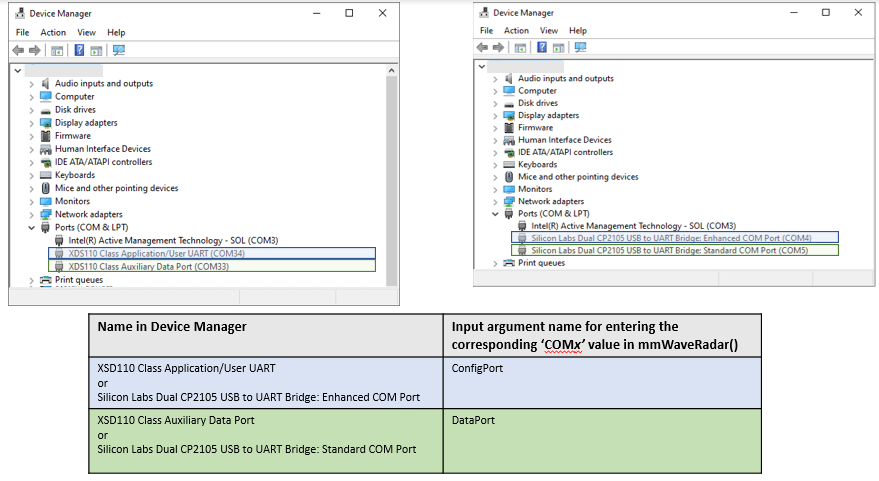
Note: The IWRL6432BOOST board uses a single port, that is, ConfigPort to download the binary, configure the radar, and acquire the data. Therefore, you need to specify only the ConfigPort value for this board.

Specify Configuration File

To configure the TI mmWave radar board, you must send a sequence of commands to the board using the serial port. The sequence includes commands specifying the chirp profile, sampling rate, required outputs, and so on. For more information on the commands, see the Configuration (.cfg) File Format section in mmWave SDK user guide. Use the ConfigFile property of the mmWaveRadar object to send the sequence of commands to the board. For example:

installDir = matlabshared.supportpkg.getSupportPackageRoot
tiradarCfgFileDir = fullfile(installDir,'toolbox','target', 'supportpackages', 'timmwaveradar', 'configfiles');
tiradar.ConfigFile = fullfile(tiradarCfgFileDir, 'xwr68xx_2Tx_BestRange_UpdateRate_10.cfg');

If the configuration file is already in the MATLAB path, specify only the filename with the extension.

The mmWaveRadar object sets a few properties of the object based on the parameters in the configuration file.

Generate Configuration File for All Supported Boards Except IWRL6432BOOST

For all the supported boards except the IWRL6432BOOST board, use mmWave Demo visualizer application to generate the configuration file.

Use the Setup Details and Scene Selection sections in the application to specify the required configurations.

Select the appropriate platform for your TI board:

xwr68xx for TI IWR6843ISK or TI AWR6843ISK
xwr68xx_AOP for TI IWR6843AOPEVM or TI AWR6843AOPEVM
xwr18xx_AOP for TI IWR1843AOPEVM
xwr16xx for TI AWR1642BOOST

Use the check boxes in Plot Selection section to specify the required outputs:

Select Scatter plot for getting detections (point cloud) outputs.
Select Range Profile and Noise Profile for getting range profile and noise profile outputs respectively.
Select Range Doppler Heat Map and Range Azimuth Heat Map for getting range doppler and range angle responses in outputs respectively .

Once you have specified the required configurations, click SAVE CONFIG TO PC to generate the corresponding .cfg file. For more information about the outputs that you obtain in MATLAB, see mmWaveRadar object.

At the default baud rate of 921600, for getting heat map outputs, set the frame rate to less than or equal to 5 fps. For more information, see Performance Considerations for Using mmWave Radar Sensors.

Generate Configuration (.cfg) File for IWRL6432BOOST

To generate the Configuration (.cfg) file for the IWRL6432BOOST, refer to Parameter Tuning and Customization Guide for the IWRL6432 Motion/Presence Detection Demo. You can find information about this guide at this link.

Use Sample Configuration Files

You can use a sample configuration file provided with the support package instead of generating a configuration file. The sample files are stored in the configfiles folder. Execute the following commands in the MATLAB Command Window to access the files.

installDir = matlabshared.supportpkg.getSupportPackageRoot
tiradarCfgFileDir = fullfile(installDir,'toolbox','target', 'supportpackages', 'timmwaveradar', 'configfiles');
cd(tiradarCfgFileDir)

Configure Radar and Start Reading the Measurements

The first call to the mmWaveRadar object after object creation or the first call to the mmWaveRadar object after calling release function, configures the device as per the Config file and properties that you set. This step also starts streaming data from radar board.

Call the mmWaveRadar object to configure the radar and to start streaming the data.

[dets, timestamp, meas, overrun] = tiradar()

The value of the timestamp output is 0 when you call the object for the first time after creating it. The object can take longer to execute the first call (than the subsequent calls to the mmWaveRadar object) as this call involves configuration and validation steps.

Note: You can call System objects directly like a function instead of using the step function. For example, y = step(obj) and y = obj() are equivalent.

You can use the object properties to configure the radar and its output characterstics. For example:

Set the EnableRangeGroups and EnableDopplerGroups properties to true to enable peak grouping in the range and Doppler directions. When you enable peak grouping, the radar reports only one (the highest) point instead of reporting a cluster of neighboring points. This reduces the total number of detected points per read.

tiradar.EnableRangeGroups = true;
tiradar.EnableDopplerGroups = true;

Set the AzimuthLimits property so that the radar does not output detections outside the specified azimuth limits.

tiradar.AzimuthLimits = [-60 60];

Use the DetectionCoordinates property to specify the coordinate system that the radar uses to report detections.

tiradar.DetectionCoordinates = "Sensor rectangular";

For more information on the supported properties and outputs, see mmWaveRadar object.

Read and Plot Position and Range Profile

You can read measurements for the TI mmWave radar and plot the radar data. The mmWaveRadar object outputs a cell array of objectDetection class objects, where each object contains an object detection report obtained by the sensor for that object. For more information, see mmWaveRadar object.

Note: Ensure that the point cloud and range profile outputs are enabled for the radar to get the correspoinding output using MATLAB function. These outputs are enabled by setting the values corresponding to pointCloud and rangeProfile parameters in the guiMonitor command in Configuration (.cfg) file. For more details, refer to guiMonitor command description in xWRL6432 MMWAVE-L-SDK: Motion and Presence Detection OOB Demo (for IWRL6432BOOST), and in the Configuration (.cfg) File Format section in MMWAVE SDK User Guide (for other supported boards).

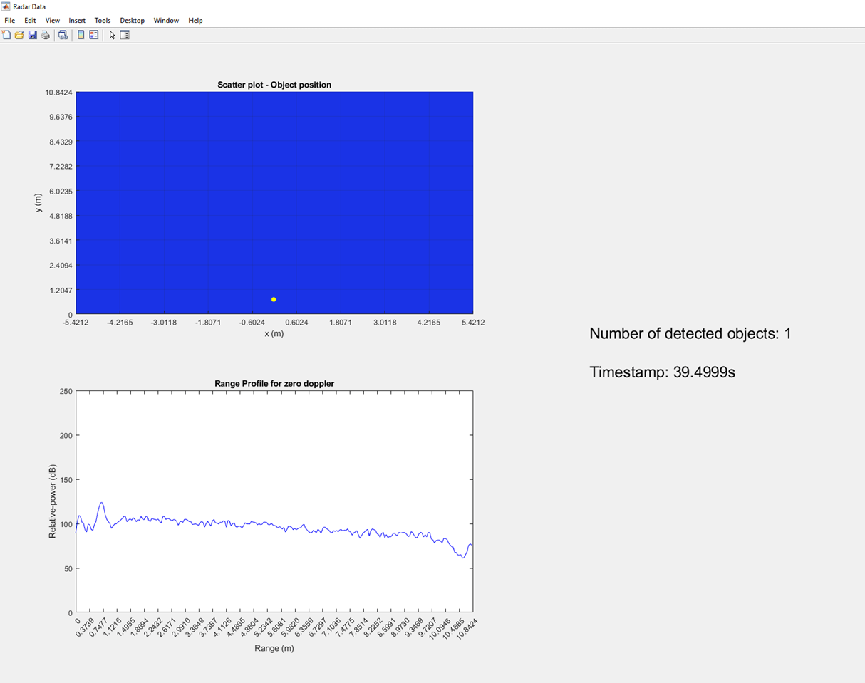
% Create mmWaveRadar object and specify its properties.
% This MATLAB code assumes that you have connected TI IWR6843ISK module to the USB port of your computer, 
% and that you had flashed the binary and set up the TI IWR6843ISK module for data acquisition using the Hardware Setup screens. 
% If you are using another board, change the input argument accordingly.
tiradar = mmWaveRadar("TI IWR6843ISK");
tiradar.AzimuthLimits = [-60 60];
tiradar.DetectionCoordinates = "Sensor rectangular";

% Create figure and other graphic objects to view the detections and range profile
fig = figure('Name','Radar Data', 'WindowState','maximized','NumberTitle','off');
tiledlayout(fig,2,2);

% Create handle to scatter plot and initialize its properties for plotting detections
ax1 = nexttile;
scatterPlotHandle = scatter(ax1,0,0,'filled','yellow');
ax1.Title.String = 'Scatter plot - Object position';
ax1.XLabel.String = 'x (m)';
ax1.YLabel.String = 'y (m)';
% Update the xlimits, ylimits and nPoints as per the scenario and Radar properties
% Y-axis limits for the scatter plot
yLimits = [0,tiradar.MaximumRange];
% X-axis limits for the scatter plot
xLimits = [-tiradar.MaximumRange/2,tiradar.MaximumRange/2];
% Number of tick marks in x and y axis in the scatter plot
nPoints = 10;
ylim(ax1,yLimits);
yticks(ax1,linspace(yLimits(1),yLimits(2),nPoints))
xlim(ax1,xLimits);
xticks(ax1,linspace(xLimits(1),xLimits(2),nPoints));
set(ax1,'color',[0.1 0.2 0.9]);
grid(ax1,'on')

% Create text handle to print the number of detections and time stamp
ax2 = nexttile([2,1]);
blnkspaces = blanks(1);
txt = ['Number of detected objects: ','Not available',newline newline,'Timestamp: ','Not available'];
textHandle = text(ax2,0.1,0.5,txt,'Color','black','FontSize',20);
axis(ax2,'off');

% Create plot handle and initialize properties for plotting range profile
ax3 = nexttile();
rangeProfilePlotHandle = plot(ax3,0,0,'blue');
ax3.Title.String = 'Range Profile for zero Doppler';
ax3.YLabel.String = 'Relative-power (dB)';
ax3.XLabel.String = 'Range (m)';
% Update the xlimits, ylimits and nPoints as per the scenario and Radar properties
% X-axis limits for the plot
xLimits = [0,tiradar.MaximumRange];
% Y-axis limits for the plot
yLimits = [0,250];
% Number of tick marks in x axis in the Range profile plot
nPoints = 30;
ylim(ax3,yLimits);
xlim(ax3,xLimits);
xticks(ax3,linspace(xLimits(1),xLimits(2),nPoints));

% Read radar measurements in a loop and plot the measurements for for 50s (specified by stopTime)
ts = tic;
stopTime = 50;
while(toc(ts)<=stopTime)
    % Read detections and other measurements from TI mmWave Radar
    [objDetsRct,timestamp,meas,overrun] = tiradar();
    % Get the number of detections read
    numDets = numel(objDetsRct);
    % Print the timestamp and number of detections in plot
    txt = ['Number of detected objects: ', num2str(numDets),newline newline,'Timestamp: ',num2str(timestamp),'s'];
    textHandle.String = txt;
    % Detections will be empty if the output is not enabled or if no object is
    % detected. Use number of detections to check if detections are available
    if numDets ~= 0
        % Detections are reported as cell array of objects of type objectDetection
        % Extract  x-y position information from each objectDetection object
        xpos = zeros(1,numDets);
        ypos = zeros(1,numDets);
        for i = 1:numel(objDetsRct)
            xpos(i) = objDetsRct{i}.Measurement(1);
            ypos(i) = objDetsRct{i}.Measurement(2);
        end
        [scatterPlotHandle.XData,scatterPlotHandle.YData] = deal(ypos,xpos);
    end
    % Range profile will be empty if the log magnitude range output is not enabled
    % via guimonitor command in config File
    if ~isempty(meas.RangeProfile)
        [rangeProfilePlotHandle.XData,rangeProfilePlotHandle.YData] = deal(meas.RangeGrid,meas.RangeProfile);
    end
    drawnow limitrate;
end
clear tiradar;

This image shows the output of the code snippet where there is only one object in front of the radar.

Read and Plot Detections Using birdsEyePlot Object

You can also use the birdsEyePlot (Automated Driving Toolbox) object from Automated Driving Toolbox™ to plot the detections that you obtained from TI mmWaveRadar sensor. You must have a license for Automated Driving Toolbox to run these commands:

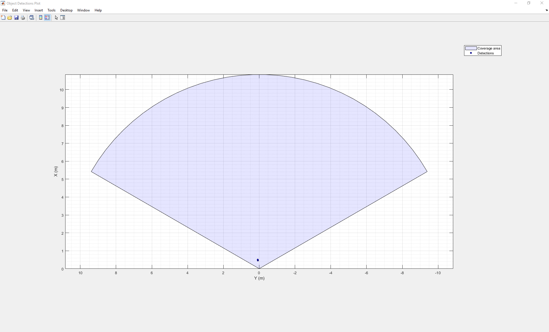
% Create mmWaveRadar object and specify its properties.
tiradar = mmWaveRadar("TI IWR6843ISK");
tiradar.AzimuthLimits = [-60 60];
tiradar.DetectionCoordinates = "Sensor rectangular";
% Close all open figures
close all
% Creates a bird's-eye plot in a new figure and initialize properties
f = figure('NumberTitle', 'off', 'Name', 'Object Detections Plot');
axBEP = axes(f);
axis(axBEP,'equal');
grid(axBEP,'on');
grid(axBEP,'minor');
cla(axBEP);
xLimits = [0,tiradar.MaximumRange];
yLimits = [-tiradar.MaximumRange,tiradar.MaximumRange];
% Create a birdsEyePlot object to displays a bird's-eye plot of a 2-D scenario to plot
% detections and sensor coverage
bep = birdsEyePlot('Parent',axBEP,'XLim',xLimits,'YLim',yLimits);
% Field of view of the sensor coverage area
azFOV = tiradar.AzimuthLimits(2)-tiradar.AzimuthLimits(1);
% Create a CoverageAreaPlotter object to configures the display of sensor coverage areas on a
% bird's-eye plot.
caPlotter = coverageAreaPlotter(bep,'DisplayName','Coverage area','FaceColor','b');
% Display sensor coverage area on bird's-eye plot
plotCoverageArea(caPlotter,tiradar.MountingLocation(1:2),tiradar.MaximumRange,tiradar.MountingAngles(1),azFOV);
%  Creates a detection plotter
detPlotter = detectionPlotter(bep,'DisplayName','Detections', 'Marker','o','MarkerFaceColor','b','MarkerSize',4);

ts = tic;
stopTime = 100;
while(toc(ts)<=stopTime)
    % Read detections and other measurements from TI mmWave Radar
    [objDetsRct,timestamp,measurements,overrun] = tiradar();
    % Get the number of detections read
    numDets = numel(objDetsRct);
    pos = zeros(3,numDets);
    vel = zeros(3,numDets);
    % Detections are reported as cell array of objects of type objectDetection
    % Extract  x-y position information from each objectDetection object
    for i = 1:numDets
        pos(:,i) = objDetsRct{i}.Measurement(1:3);
        vel(:,i) = objDetsRct{i}.Measurement(4:6);
    end
    % Displays detections and their velocities on a bird's-eye plot.
    plotDetection(detPlotter,pos',vel');
    drawnow limitrate;
end
clear tiradar

This image shows the output of the code snippet where there is only one object in front of the radar.

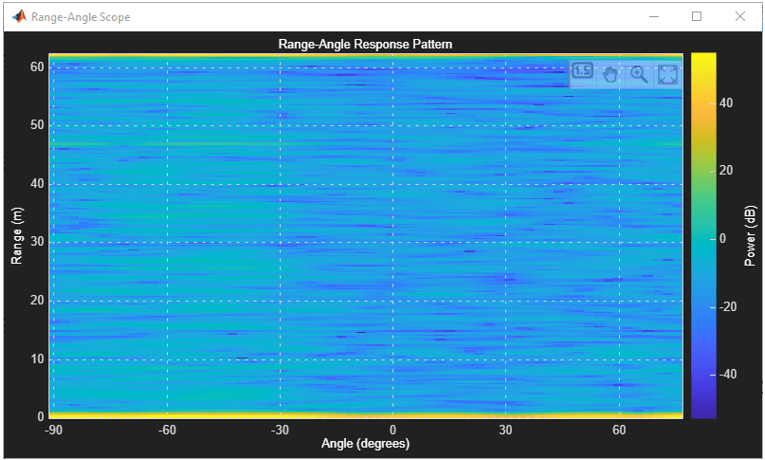
Read and Plot Range Doppler Response and Range Azimuth Response

You can plot range Doppler response and range azimuth response that is read from the TI mmWave radar. Because the range Doppler response and range azimuth response data are large in size, use an update rate of less than 5Hz. For more information on performance, see Performance Considerations for Using mmWave Radar Sensors.

Note: Ensure that the range doppler response and range Azimuth response are enabled for the radar to get the correspoinding output using MATLAB function. These outputs are enabled by setting the values corresponding to pointCloud and rangeProfile parameters in the guiMonitor command in Configuration (.cfg) file. For more details, refer to guiMonitor command description in xWRL6432 MMWAVE-L-SDK: Motion and Presence Detection OOB Demo (for IWRL6432BOOST), and in the Configuration (.cfg) File Format section in MMWAVE SDK User Guide (for other supported boards).

Note: Range-Doppler response and range azimuth response are not supported for IWRL6432BOOST board. Range azimuth response is not supported for IWR6843AOPEVM, AWR6843AOPEVM, and AWR1843AOPEVM boards.

To change the update rate, the corresponding parameter in the Configuration (.cfg) file needs to be updated. To change the Configuration file, stop the sensor and release the properties by invoking release method, and then use the property ConfigFile to update the config file.

% Create mmWaveRadar object and specify its properties.
tiradar = mmWaveRadar("TI IWR6843ISK");
% Use Config file which configures sensor to output range Angle and range Doppler 
% response and has Update rate less than 5 Hz.
installDir = matlabshared.supportpkg.getSupportPackageRoot;
tiradarCfgFileDir = fullfile(installDir,'toolbox','target', 'supportpackages', 'timmwaveradar', 'configfiles');
tiradar.ConfigFile = fullfile(tiradarCfgFileDir,'xwr68xx_2Tx_UpdateRate_1.cfg');

Start the sensor by invoking the first step function and read and plot range Doppler and range angle response.

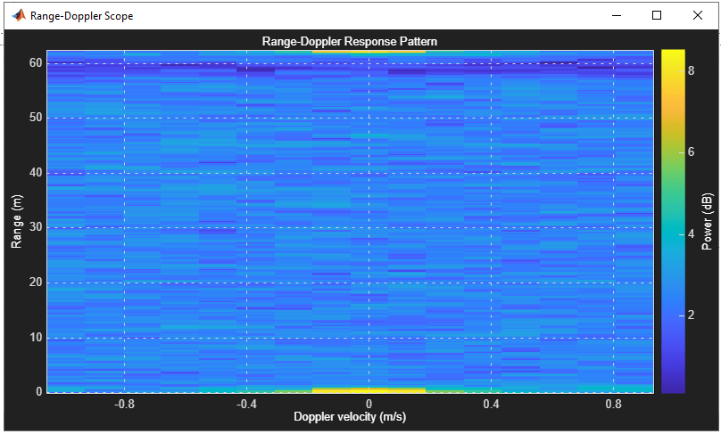
% Configure and start the sensor by invoking the first step function
tiradar();
% Creates a scope for viewing a range- Angle response map
rngAngleScope = phased.RangeAngleScope;
%  The input data to scope is response data that has already been
%  processed, set IQDataInput as false
rngAngleScope.IQDataInput = false;
% Creates a scope for viewing a range- Doppler response map
rngDopplerScope = phased.RangeDopplerScope;
%  The input data to scope is response data that has already been
%  processed, set IQDataInput as false
rngDopplerScope.IQDataInput = false;
rngDopplerScope.DopplerLabel = 'Doppler velocity (m/s)';

% Read and view the responses in the Range angle and Range Doppler Scope 
ts = tic;
stopTime = 10;
while(toc(ts)<=stopTime)
    [dets,timestamp,meas,overrun] = tiradar();
    % meas.RangeDopplerResponse will be empty, if the rangeDopplerHeatMap output is not enabled
    % via guimonitor command in config file
    if ~isempty(meas.RangeDopplerResponse)
        %  Displays a range-Doppler response map, at the ranges
        %  Doppler shifts specified
        rngDopplerScope(meas.RangeDopplerResponse,meas.RangeGrid',meas.DopplerGrid')
    end
    % meas.RangeAngleResponse will be empty, if the rangeAzimuthHeatMap output is not enabled
    % via guimonitor command in config file
    if ~isempty(meas.RangeAngleResponse)
        rngAngleScope(meas.RangeAngleResponse,meas.RangeGrid',meas.AngleGrid')
    end
    drawnow limitrate;
end

This image shows the output of the code snippet when the radar antenna is covered.

Stop the radar sensor from sending data and clear the mmWaveRadar object.

tiradar.release();
clear tiradar

Close all figures.

close all