Automatic Data Segmentation and Feature Extraction for Reference Performance Test in Lab-Measured Battery Aging Data
R2026bReference performance tests (RPT) are included in battery aging test design when there is no unified measurement available for obtaining remaining capacity or when additional measurements (slow rate cycles, pulses, EIS, etc.) are needed to characterize the battery's health. This example illustrates the use of a neural network for separating current pulses from regular charge-discharge steps and the extraction of features, that serve as health indicators, from the identified pulses.
Battery RPT data
The data used in this example is from one cell in ISU-ILCC Battery Aging Dataset [1], and is preprocessed to only contain raw measurements from RPTs (i.e., the cycling test data are excluded). The type of cell used in this dataset is NMC/graphite pouch cell with a rated capacity of 0.25Ah (1C = 0.25A). The RPT were performed using a 64-channel Neware BTS4000 series battery tester with cells placed in a temperature-controlled chamber set at 30°C. For this example, the essential measurements are:
RPT_Index - An integer identifying the RPT test number (starting from 1).
Steps - An integer identifying a step within the RPT profile (starting from 1).
Current (A) - The current measured in Amps.
Voltage (V) - The terminal voltage measured in Volts.
Capacity (Ah) - The cumulative charge/discharge capacity in a step measured in Amp-hour.
Relative Time (h:min:s.ms) - The time stamps relative to the start of each step.
Real Time (h:min:s.ms) - The time stamps with date and time.
Download the data from the MathWorks support files site and load it into MATLAB.
url = 'https://ssd.mathworks.com/supportfiles/predmaint/batteryagingdata/isuilcc/rpt/RPT_ISU_ILCC.zip';
downloadFolder = fullfile(tempdir,tempname);
loc = websave('BatteryRPTDataset', url);
unzip(loc, pwd)

load("RPT_ISU.mat","data")
head(data)
    RPT_Index    Record number     status      Jump    Cycle    Steps    Current(A)    Voltage(V)    Capacity(Ah)    Energy(Wh)    Relative Time(h:min:s.ms)     Real Time(h:min:s.ms)
    _________    _____________    _________    ____    _____    _____    __________    __________    ____________    __________    _________________________    _______________________

        1              1          "CC DChg"     1        1        1        -0.05         4.0119                0              0          00:00:00.000           2022-09-16 20:13:49.000
        1              2          "CC DChg"     1        1        1        -0.05         4.0091       6.9437e-05     0.00027847          00:00:05.000           2022-09-16 20:13:54.000
        1              3          "CC DChg"     1        1        1        -0.05         4.0073       0.00013888     0.00055682          00:00:10.000           2022-09-16 20:13:59.000
        1              4          "CC DChg"     1        1        1        -0.05          4.006       0.00020833     0.00083505          00:00:15.000           2022-09-16 20:14:04.000
        1              5          "CC DChg"     1        1        1        -0.05         4.0051       0.00027777      0.0011132          00:00:20.000           2022-09-16 20:14:09.000
        1              6          "CC DChg"     1        1        1        -0.05         4.0042       0.00034721      0.0013913          00:00:25.000           2022-09-16 20:14:14.000
        1              7          "CC DChg"     1        1        1        -0.05         4.0032       0.00041666      0.0016693          00:00:30.000           2022-09-16 20:14:19.000
        1              8          "CC DChg"     1        1        1        -0.05         4.0026        0.0004861      0.0019473          00:00:35.000           2022-09-16 20:14:24.000
Visualize the Data from One RPT
To better understand the RPT profile design in this dataset, visualize the current and voltage measurements from one RPT. At the beginning, the cells are discharged to 3V with C/5 current. Then, a sequence of a C/5 full-depth cycle, a C/2 full-depth cycle with pulses during discharge, and a C/2 full-depth cycle is performed. Plot the current, voltage, and time from the second RPT Test.
dataCycle = data(data.RPT_Index==2,:);

currentCycle = dataCycle.("Current(A)");
voltageCycle = dataCycle.("Voltage(V)");
timeCycle = dataCycle.("Real Time(h:min:s.ms)");
relTimeCycle = seconds(timeCycle - timeCycle(1));

figure()
yyaxis left
plot(relTimeCycle,currentCycle,LineWidth=1.5)
ylabel("Current (A)")
yyaxis right
plot(relTimeCycle,voltageCycle,LineWidth=1.5)
ylabel("Voltage (V)")
xlabel("Time (sec)")
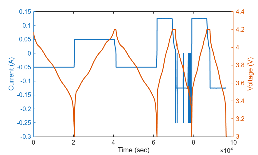
Zooming in to the first pulse in the RPT, it can be seen that when a discharge pulse is injected, the terminal voltage of the cell dips in response. Select 5 seconds before and after the pulse and plot the current and voltage for this duration.
dataPulse = dataCycle(ismember(dataCycle.Steps,[9,10,11]),:);
timePulse = dataPulse.("Real Time(h:min:s.ms)");
timePulseDur = timePulse - timePulse(1);

idx = timePulseDur<=duration(0,0,20)&timePulseDur>=duration(0,0,5);
relTimePulse = seconds(timePulseDur(idx))-5; % Offset by 5 seconds
currentPulse = dataPulse(idx,"Current(A)").("Current(A)");
voltagePulse = dataPulse(idx,"Voltage(V)").("Voltage(V)");

figure()
yyaxis left
plot(relTimePulse,currentPulse,LineWidth=1.5)
ylabel("Current (A)")
ylim([-0.3,0])
yyaxis right
plot(relTimePulse,voltagePulse,LineWidth=1.5)
ylabel("Voltage (V)")
xlabel("Time (sec)")
xlim([0,max(relTimePulse)])
ylim([4.12,4.2])
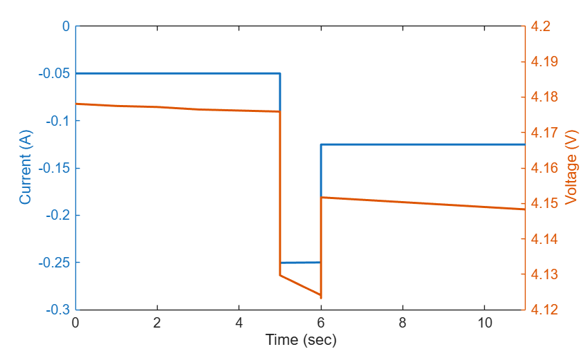
As the cell ages, the magnitude and pattern of this voltage dip could change, which provides useful information regarding the degradation. Thus, it is useful to extract features from these measurements and track changes in these features over cycles. However, as seen above, an RPT can contain both charge-discharge cycles and pulses. It is time consuming to manually extract the segments associated with the pulses. So, in the next section, a neural network is trained to identify pulses in an RPT measurement and the trained network is then used to identify all the pulses for feature extraction.
Train a Neural Network to Perform Automatic Segmentation
A bi-directional long short-term memory (BiLSTM) model is trained to perform automatic segmentation. Assume that the data is partially labeled, and train the BiLSTM model on the available labeled data. Use the trained model to label the remaining unlabeled data.
Load predefined labels for a portion of the RPT data and append to the data table. Each point is labeled to be a part of a Pulse or Regular charge-discharge cycle. Points that are neither are not labeled and have an "undefined" label.
load("RPT_ISU_label.mat","label")
data.Label = label;
head(data)
    RPT_Index    Record number     status      Jump    Cycle    Steps    Current(A)    Voltage(V)    Capacity(Ah)    Energy(Wh)    Relative Time(h:min:s.ms)     Real Time(h:min:s.ms)        Label
    _________    _____________    _________    ____    _____    _____    __________    __________    ____________    __________    _________________________    _______________________    ___________

        1              1          "CC DChg"     1        1        1        -0.05         4.0119                0              0          00:00:00.000           2022-09-16 20:13:49.000    <undefined>
        1              2          "CC DChg"     1        1        1        -0.05         4.0091       6.9437e-05     0.00027847          00:00:05.000           2022-09-16 20:13:54.000    <undefined>
        1              3          "CC DChg"     1        1        1        -0.05         4.0073       0.00013888     0.00055682          00:00:10.000           2022-09-16 20:13:59.000    <undefined>
        1              4          "CC DChg"     1        1        1        -0.05          4.006       0.00020833     0.00083505          00:00:15.000           2022-09-16 20:14:04.000    <undefined>
        1              5          "CC DChg"     1        1        1        -0.05         4.0051       0.00027777      0.0011132          00:00:20.000           2022-09-16 20:14:09.000    <undefined>
        1              6          "CC DChg"     1        1        1        -0.05         4.0042       0.00034721      0.0013913          00:00:25.000           2022-09-16 20:14:14.000    <undefined>
        1              7          "CC DChg"     1        1        1        -0.05         4.0032       0.00041666      0.0016693          00:00:30.000           2022-09-16 20:14:19.000    <undefined>
        1              8          "CC DChg"     1        1        1        -0.05         4.0026        0.0004861      0.0019473          00:00:35.000           2022-09-16 20:14:24.000    <undefined>
To prepare the data for training, process the data using the helper function hProcessClassificationData into two cell variables, X and Y. The measured signal is returned as X and it is a cell array with 37 elements and each cell contains a two-row matrix. The first row is current, and the second row is voltage. The labels for each measured signal cell is returned as Y, which is also a 37 element cell array, with each cell being a categorical vector for the labels ("Regular" and "Pulse").
[X, Y] = hProcessClassficationData(data);
Visualize the preprocessed data for neural network training.
currentPlot = X{2}(1,:);
voltagePlot = X{2}(2,:);
classes = categories(Y{2});

hPlotLabeledSignals(currentPlot, voltagePlot, classes, Y)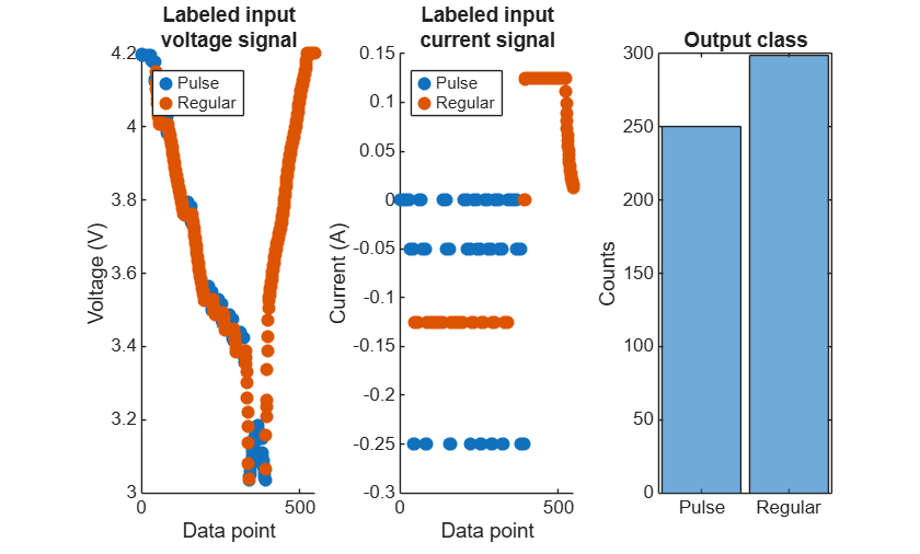
As seen in the above plots, voltage data by it self is not very different between the regular and pulse classes because the cell has to operate within its nominal range. However, the current data is clearly differentiated between the pulse and the regular classes. Thereby the combination of the current and voltage data as predictors can achieve good segmentation results. Further, the training data has been processed to balance the number of data points for regular and pulse classes to ensure a good fit.
Select 70% of RPTs for training using cvpartition function and use hTrainSegmentModel helper function to define and train the neural network.
rng default

cv = cvpartition(max(data.RPT_Index),"HoldOut",0.3);

idxTrain = training(cv);
Xtrain = X(idxTrain,1);
Ytrain = Y(idxTrain,1);

net = hTrainSegmentModel(Xtrain,Ytrain);
Training on single CPU.
|========================================================================================|
|  Epoch  |  Iteration  |  Time Elapsed  |  Mini-batch  |  Mini-batch  |  Base Learning  |
|         |             |   (hh:mm:ss)   |   Accuracy   |     Loss     |      Rate       |
|========================================================================================|
|       1 |           1 |       00:00:00 |       44.37% |       0.6741 |          0.0010 |
|      50 |          50 |       00:00:04 |       87.23% |       0.3225 |          0.0010 |
|     100 |         100 |       00:00:09 |       98.52% |       0.0449 |          0.0010 |
|========================================================================================|
Training finished: Max epochs completed.
Classify All Steps Using This Trained Model
The trained neural network can classify each data point. Given that one step can only associate to one class (i.e., a step is either "Regular" or "Pulse"), apply majority voting for each step to correct possible misclassifications at the beginning/end of the step. Use the helper function hRptDataParser to label each step as either "Regular" or "Pulse". The neural network model only classifies the step before the current pulse. So, the index for the step after pulses needs to be added explicitly after the model completes the segmentation.
segmentedData = hRptDataParser(data,net);
head(segmentedData)
    RPT_Index    Record number     status      Jump    Cycle    Steps    Current(A)    Voltage(V)    Capacity(Ah)    Energy(Wh)    Relative Time(h:min:s.ms)     Real Time(h:min:s.ms)        Label       Individual_class    Step_class
    _________    _____________    _________    ____    _____    _____    __________    __________    ____________    __________    _________________________    _______________________    ___________    ________________    __________

        1              1          "CC DChg"     1        1        1        -0.05         4.0119                0              0          00:00:00.000           2022-09-16 20:13:49.000    <undefined>         Pulse           Regular
        1              2          "CC DChg"     1        1        1        -0.05         4.0091       6.9437e-05     0.00027847          00:00:05.000           2022-09-16 20:13:54.000    <undefined>         Pulse           Regular
        1              3          "CC DChg"     1        1        1        -0.05         4.0073       0.00013888     0.00055682          00:00:10.000           2022-09-16 20:13:59.000    <undefined>         Pulse           Regular
        1              4          "CC DChg"     1        1        1        -0.05          4.006       0.00020833     0.00083505          00:00:15.000           2022-09-16 20:14:04.000    <undefined>         Pulse           Regular
        1              5          "CC DChg"     1        1        1        -0.05         4.0051       0.00027777      0.0011132          00:00:20.000           2022-09-16 20:14:09.000    <undefined>         Pulse           Regular
        1              6          "CC DChg"     1        1        1        -0.05         4.0042       0.00034721      0.0013913          00:00:25.000           2022-09-16 20:14:14.000    <undefined>         Pulse           Regular
        1              7          "CC DChg"     1        1        1        -0.05         4.0032       0.00041666      0.0016693          00:00:30.000           2022-09-16 20:14:19.000    <undefined>         Pulse           Regular
        1              8          "CC DChg"     1        1        1        -0.05         4.0026        0.0004861      0.0019473          00:00:35.000           2022-09-16 20:14:24.000    <undefined>         Pulse           Regular
Extract Features from Pulses
Use the batteryPulseFeatures function to automatically identify pulse segments and extract features from each RPT cycle. The function detects pulses based on constant-current segments and step indices, then computes the following features for each identified pulse:
OCV - Open circuit voltage before the pulse ()
R0 - Ohmic resistance (), representing the instantaneous voltage drop due to internal resistance
RTotal - Total resistance (), including both ohmic and polarization effects
DeltaVoltage - Total voltage change from pre-pulse equilibrium to end of recovery period
RelaxationVoltage - Voltage at end of relaxation period ()
RecoveryVoltage - Voltage at the start of the recovery period immediately after pulse ends
RecoveryRate - Rate of voltage recovery during relaxation (V/s)
Energy - Cumulative energy dissipated during the pulse (J)
VoltageMean - Mean voltage during the pulse period
VoltageStandardDeviation - Standard deviation of voltage during the pulse period
featureTable = table();
for cycle = unique(segmentedData.RPT_Index)'
    dataCycle = segmentedData(segmentedData.RPT_Index == cycle, :);
    [ft, pulses] = batteryPulseFeatures(dataCycle, ...
        "CurrentVariable", "Current(A)", ...
        "VoltageVariable", "Voltage(V)", ...
        "StepIndexVariable", "Steps", ...
        "ValidPulseDurationRange", [1, 30], ...
        "TimeVariable", "Relative Time(h:min:s.ms)");
    ft.Cycle_Index = repmat(cycle, height(ft), 1);
    ft.Step_Index = pulses.PulseStepIndex;
    featureTable = [featureTable; ft];
end
head(featureTable)
     OCV        R0       RTotal     DeltaVoltage    RelaxationVoltage    RecoveryVoltage    RecoveryRate      Energy      VoltageMean    VoltageStandardDeviation    Cycle_Index    Step_Index
    ______    _______    _______    ____________    _________________    _______________    ____________    __________    ___________    ________________________    ___________    __________

    4.1759      0.265      0.265        0.066            4.1099              4.1514         -0.00046111     0.00028649      4.1254              0.0035355                 1             10
    4.0296     0.2495     0.2495       0.0357            3.9939              4.0076         -0.00015222     0.00027649      3.9814              0.0024042                 1             14
    3.7837     0.2445     0.2445       0.0341            3.7496               3.763         -0.00014889     0.00025947      3.7363               0.002192                 1             18
    3.5509     0.2665     0.2665       0.0347            3.5162              3.5292         -0.00014444     0.00024306      3.5001              0.0035355                 1             22
    3.5159    0.26499    0.27449       0.0372            3.4787              3.4926         -0.00015444     0.00024054      3.4641              0.0038991                 1             26
    3.4747     0.2825    0.29931       0.0413            3.4334               3.448         -0.00016222      0.0002375      3.4188              0.0043844                 1             30
    3.4238     0.2885    0.34849       0.0601            3.3637              3.3875         -0.00026444      0.0002335      3.3632              0.0081695                 1             34
    3.2093    0.31529    0.62368       0.0958            3.3051              3.1017             0.00678     0.00021727      3.1263               0.027926                 1             38
To estimate the health of the cell, use the helper function hFindCapacity to calculate the remaining capacity of the cell and capacity loss at each RPT.
[capacity,capacityLoss] = hFindCapacity(segmentedData);
capacityTable = array2table([capacity,capacityLoss],...
    'VariableNames',["Remaining_Capacity","Capacity_Loss"]);
head(capacityTable)
    Remaining_Capacity    Capacity_Loss
    __________________    _____________

         0.28524                    0
         0.28411            0.0011261
         0.28285            0.0023864
         0.27962            0.0056198
         0.27672              0.00852
         0.27418             0.011059
         0.27213             0.013109
         0.27008             0.015162
Plot the extracted features to visualize any trends that indicate correlation with aging. Select pulse step 18 to track features across RPT cycles. The DeltaVoltage feature represents the total voltage drop from pre-pulse equilibrium to end of recovery, and R0 is the ohmic resistance. Both increase as the battery degrades.
stepIndex = 18;
featureCycle = featureTable(featureTable.Step_Index == stepIndex, :);
rptFeaturesToPlot = ["DeltaVoltage","R0"];

for iii = 1:length(rptFeaturesToPlot)
    figure()
    yyaxis left
    plot(featureCycle.Cycle_Index, featureCycle.(rptFeaturesToPlot(iii)), '-o', LineWidth=1.5)
    xlabel('RPT Index')
    ylabel(rptFeaturesToPlot(iii),Interpreter="none")
    yyaxis right
    plot(capacityTable,"Capacity_Loss")
    ylabel('Capacity loss(Ah)')
end
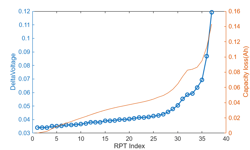
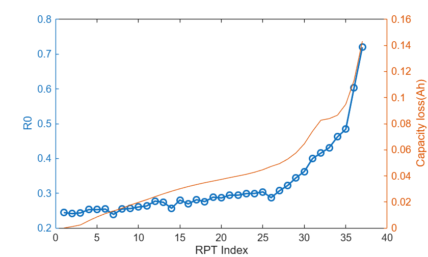
The trends of these features as cell ages align with the capacity loss, but the evolution of feature values is not smooth as the capacity loss. The main reason is that the current pulse in this dataset is only applied for 1 seconds, which is a very short period of time so that cell is still in transient state. This will result in higher noise in the feature extraction because the measurements can be taken at different stage of the transient state.
Conclusion
This example illustrates automatic segmentation of pulses from battery reference performance tests using deep learning. Automatic data segmentation reduces the need for manual intermediate data processing to extract pulse or other type of test components (e.g., EIS). Synthetic data simulated from physics-based models could be used to expand the capability of such deep learning models for more complicated RPT designs, such as a blend of charge and discharge pulses.
The batteryPulseFeatures function was used to automatically identify pulse segments and extract key health indicators such as ohmic resistance, total resistance, and voltage drop. These features show strong correlation with the capacity loss as the cell ages and can be used as predictors of state of health or other battery health indicators.
[1] Thelen, Adam; Li, Tingkai; Liu, Jinqiang; Tischer, Chad; Hu, Chao (2023). ISU-ILCC Battery Aging Dataset. Iowa State University. Dataset. https://doi.org/10.25380/iastate.22582234.v2

