Electronic Scanning Using a Uniform Rectangular Array
This example simulates a phased array radar that periodically scans a predefined surveillance region. A 900-element rectangular array is used in this monostatic radar. Steps are introduced to derive the radar parameters according to specifications. After synthesizing the received pulses, detection and range estimation are performed. Finally, Doppler estimation is used to obtain the speed of each target.
Radar Definition
First we create a phased array radar. We reuse most of the subsystems built in the example Simulating Test Signals for a Radar Receiver. Readers are encouraged to explore the details of radar system design through that example. A major difference is that we use a 30-by-30 uniform rectangular array (URA) in place of the original single antenna.
The existing radar design meets the following specifications.
pd = 0.9;            % Probability of detection
pfa = 1e-6;          % Probability of false alarm
max_range = 5000;    % Maximum unambiguous range
tgt_rcs = 1;         % Required target radar cross section
int_pulsenum = 10;   % Number of pulses to integrate
Load the radar system and retrieve system parameters.
load BasicMonostaticRadarExampleData;

fc = radiator.OperatingFrequency;         % Operating frequency (Hz)
v = radiator.PropagationSpeed;            % Wave propagation speed (m/s)
lambda = v/fc;                            % Wavelength (m)
fs = waveform.SampleRate;                 % Sampling frequency (Hz)
prf = waveform.PRF;                       % Pulse repetition frequency (Hz)
Next, we define a 30-by-30 uniform rectangular array.
ura = phased.URA('Element',antenna,...
    'Size',[30 30],'ElementSpacing',[lambda/2, lambda/2]);
% Configure the antenna elements such that they only transmit forward
ura.Element.BackBaffled = true;

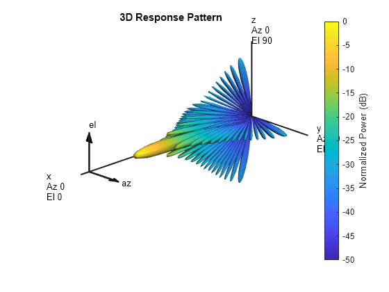
% Visualize the response pattern.
pattern(ura,fc,'PropagationSpeed',physconst('LightSpeed'),...
    'Type','powerdb');

Associate the array with the radiator and collector.
radiator.Sensor = ura;
collector.Sensor = ura;

% We need to set the WeightsInputPort property to true to enable it to
% accept transmit beamforming weights
radiator.WeightsInputPort = true;
Now we need to recalculate the transmit power. The original transmit power was calculated based on a single antenna. For a 900-element array, the power required for each element is much less.
% Calculate the array gain
arraygain = phased.ArrayGain('SensorArray',ura,'PropagationSpeed',v);
ag = arraygain(fc,[0;0]);

% Calculate the peak power
snr_min = albersheim(pd, pfa, int_pulsenum);
peak_power = ((4*pi)^3*noisepow(1/waveform.PulseWidth)*max_range^4*...
    db2pow(snr_min))/(db2pow(2*(transmitter.Gain+ag))*tgt_rcs*lambda^2)
peak_power =
0.0065
The new peak power is 0.0065 Watts.
% Set the peak power of the transmitter
transmitter.PeakPower = peak_power;
We also need to design the scanning schedule of the phased array. To simplify the example, we only search in the azimuth dimension. We require the radar to search from 45 degrees to -45 degrees in azimuth. The revisit time should be less than 1 second, meaning that the radar should revisit the same azimuth angle within 1 second.
initialAz = 45; endAz = -45;
volumnAz = initialAz - endAz;
To determine the required number of scans, we need to know the beamwidth of the array response. We use an empirical formula to estimate the 3-dB beamwidth.
where is the array gain and is the 3-dB beamwidth.
% Calculate 3-dB beamwidth
theta = radtodeg(sqrt(4*pi/db2pow(ag)))
theta = 6.7703
The 3-dB beamwidth is 6.77 degrees. To allow for some beam overlap in space, we choose the scan step to be 6 degrees.
scanstep = -6;
scangrid = initialAz+scanstep/2:scanstep:endAz;
numscans = length(scangrid);
pulsenum = int_pulsenum*numscans;

% Calculate revisit time
revisitTime = pulsenum/prf
revisitTime = 0.0050
The resulting revisit time is 0.005 second, well below the prescribed upper limit of 1 second.
Target Definition
We want to simulate the pulse returns from two non-fluctuating targets, both at 0 degrees elevation. The first target is approaching to the radar, while the second target is moving away from the radar.
tgtpos = [[3532.63; 800; 0],[2020.66; 0; 0]];
tgtvel = [[-100; 50; 0],[60; 80; 0]];
tgtmotion = phased.Platform('InitialPosition',tgtpos,'Velocity',tgtvel);

tgtrcs = [1.6 2.2];
target = phased.RadarTarget('MeanRCS',tgtrcs,'OperatingFrequency',fc);

% Calculate the range, angle, and speed of the targets
[tgtrng,tgtang] = rangeangle(tgtmotion.InitialPosition,...
    sensormotion.InitialPosition);

numtargets = length(target.MeanRCS);
Pulse Synthesis
Now that all subsystems are defined, we can proceed to simulate the received signals. The total simulation time corresponds to one pass through the surveillance region. Because the reflected signals are received by an array, we use a beamformer pointing to the steering direction to obtain the combined signal.
% Create the steering vector for transmit beamforming
steeringvec = phased.SteeringVector('SensorArray',ura,...
    'PropagationSpeed',v);

% Create the receiving beamformer
beamformer = phased.PhaseShiftBeamformer('SensorArray',ura,...
    'OperatingFrequency',fc,'PropagationSpeed',v,...
    'DirectionSource','Input port');

% Define propagation channel for each target
channel = phased.FreeSpace(...
    'SampleRate',fs,...
    'TwoWayPropagation',true,...
    'OperatingFrequency',fc);

fast_time_grid = unigrid(0, 1/fs, 1/prf, '[)');

% Pre-allocate array for improved processing speed
rxpulses = zeros(numel(fast_time_grid),pulsenum);

for m = 1:pulsenum

    % Update sensor and target positions
    [sensorpos,sensorvel] = sensormotion(1/prf);
    [tgtpos,tgtvel] = tgtmotion(1/prf);

    % Calculate the target angles as seen by the sensor
    [tgtrng,tgtang] = rangeangle(tgtpos,sensorpos);

    % Calculate steering vector for current scan angle
    scanid = floor((m-1)/int_pulsenum) + 1;
    sv = steeringvec(fc,scangrid(scanid));
    w = conj(sv);

    % Form transmit beam for this scan angle and simulate propagation
    pulse = waveform();
    [txsig,txstatus] = transmitter(pulse);
    txsig = radiator(txsig,tgtang,w);
    txsig = channel(txsig,sensorpos,tgtpos,sensorvel,tgtvel);

    % Reflect pulse off of targets
    tgtsig = target(txsig);

    % Beamform the target returns received at the sensor
    rxsig = collector(tgtsig,tgtang);
    rxsig = receiver(rxsig,~(txstatus>0));
    rxpulses(:,m) = beamformer(rxsig,[scangrid(scanid);0]);
end
Matched Filter
To process the received signal, we first pass it through a matched filter, then integrate all pulses for each scan angle.
% Matched filtering
matchingcoeff = getMatchedFilter(waveform);
matchedfilter = phased.MatchedFilter(...
    'Coefficients',matchingcoeff,...
    'GainOutputPort',true);
[mf_pulses, mfgain] = matchedfilter(rxpulses);
mf_pulses = reshape(mf_pulses,[],int_pulsenum,numscans);

matchingdelay = size(matchingcoeff,1)-1;
sz_mfpulses = size(mf_pulses);
mf_pulses = [mf_pulses(matchingdelay+1:end) zeros(1,matchingdelay)];
mf_pulses = reshape(mf_pulses,sz_mfpulses);

% Pulse integration
int_pulses = pulsint(mf_pulses,'noncoherent');
int_pulses = squeeze(int_pulses);

% Visualize
r = v*fast_time_grid/2;
X = r'*cosd(scangrid); Y = r'*sind(scangrid);
clf;
pcolor(X,Y,pow2db(abs(int_pulses).^2));
axis equal tight
shading interp
axis off
text(-800,0,'Array');
text((max(r)+10)*cosd(initialAz),(max(r)+10)*sind(initialAz),...
    [num2str(initialAz) '^o']);
text((max(r)+10)*cosd(endAz),(max(r)+10)*sind(endAz),...
    [num2str(endAz) '^o']);
text((max(r)+10)*cosd(0),(max(r)+10)*sind(0),[num2str(0) '^o']);
colorbar;

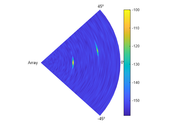
From the scan map, we can clearly see two peaks. The close one is at around 0 degrees azimuth, the remote one at around 10 degrees in azimuth.
Detection and Range Estimation
To obtain an accurate estimation of the target parameters, we apply threshold detection on the scan map. First we need to compensate for signal power loss due to range by applying time varying gains to the received signal.
range_gates = v*fast_time_grid/2;
tvg = phased.TimeVaryingGain(...
    'RangeLoss',2*fspl(range_gates,lambda),...
    'ReferenceLoss',2*fspl(max(range_gates),lambda));
tvg_pulses = tvg(mf_pulses);

% Pulse integration
int_pulses = pulsint(tvg_pulses,'noncoherent');
int_pulses = squeeze(int_pulses);

% Calculate the detection threshold

% sample rate is twice the noise bandwidth in the design system
noise_bw = receiver.SampleRate/2;
npower = noisepow(noise_bw,...
    receiver.NoiseFigure,receiver.ReferenceTemperature);
threshold = npower * db2pow(npwgnthresh(pfa,int_pulsenum,'noncoherent'));
% Increase the threshold by the matched filter processing gain
threshold = threshold * db2pow(mfgain);
We now visualize the detection process. To better represent the data, we only plot range samples beyond 50.
N = 51;
clf;
surf(X(N:end,:),Y(N:end,:),...
    pow2db(abs(int_pulses(N:end,:)).^2));
hold on;
mesh(X(N:end,:),Y(N:end,:),...
    pow2db(threshold*ones(size(X(N:end,:)))),'FaceAlpha',0.8);
view(0,56);
axis off

There are two peaks visible above the detection threshold, corresponding to the two targets we defined earlier. We can find the locations of these peaks and estimate the range and angle of each target.
[~,peakInd] = findpeaks(int_pulses(:),'MinPeakHeight',sqrt(threshold));
[rngInd,angInd] = ind2sub(size(int_pulses),peakInd);
est_range = range_gates(rngInd); % Estimated range
est_angle = scangrid(angInd);    % Estimated direction
Doppler Estimation
Next, we want to estimate the Doppler speed of each target. For details on Doppler estimation, refer to the example Doppler Estimation.
for m = numtargets:-1:1
    [p, f] = periodogram(mf_pulses(rngInd(m),:,angInd(m)),[],256,prf, ...
                'power','centered');
    speed_vec = dop2speed(f,lambda)/2;

    spectrum_data = p/max(p);
    [~,dop_detect1] = findpeaks(pow2db(spectrum_data),'MinPeakHeight',-5);
    sp(m) = speed_vec(dop_detect1); % Estimated Doppler speed
end
Finally, we have estimated all the parameters of both detected targets. Below is a comparison of the estimated and true parameter values.
------------------------------------------------------------------------
               Estimated (true) target parameters
------------------------------------------------------------------------
                 Range (m)       Azimuth (deg)   Speed (m/s)
Target 1:    3625.00 (3622.08)   12.00 (12.76)   86.01 (86.49)
Target 2:    2025.00 (2020.66)    0.00 (0.00)   -59.68 (-60.00)
Summary
In this example, we showed how to simulate a phased array radar to scan a predefined surveillance region. We illustrated how to design the scanning schedule. A conventional beamformer was used to process the received multi-channel signal. The range, angle, and Doppler information of each target are extracted from the reflected pulses. This information can be used in further tasks such as high resolution direction-of-arrival estimation, or target tracking.