Direction of Arrival Estimation Using Sparse Arrays
Direction of arrival (DOA) estimation is an important application for a sensor array. However, an N-element uniform linear array (ULA) can only resolve N-1 uncorrelated signal sources, which is a significant limitation for many applications. As a result, sparse arrays have attracted a lot of interests because you can achieve a larger array aperture with a given number of sensors. This example constructs several popular sparse array architectures and shows how they can be used to perform DOA estimation.
For the sake of simplicity, the example focuses on linear arrays. Assume there are 5 signal sources.
theta_az=[-45,-20,0,20,40]; % azimuth
Nsig = length(theta_az); % the number of target
Minimum Redundancy Array
One of the earliest sparse array designs is minimum redundancy array (MRA). An MRA is designed to provide maximum resolution for a given number of elements in the array. The idea behind an MRA is to use true elements to measure the phase difference with unique element spacing. Then using these phase shifts, we can recover the phase shifts incurred from a full size uniform linear array.
For example, let us consider a 4-element linear array, which is less than the number of signals in our scene. For a 4-element MRA, the element position is given by
d = 0.5;  % element spacing in wavelength
pos_mra = [0 1 4 6]*d;
This MRA geometry is shown in the following figure.
helperDisplayArray(pos_mra,'MRA');
It is well known that when a signal arrives at a uniform linear array, it introduces constant phase difference between adjacent sensor elements. Therefore, the correlation between two sensor elements in the array is spacing invariant, i.e., the correlation between the two sensor elements only depends on the spacing between the two sensor elements. First, let us explore what these redundancies look like for the chosen MRA.
pos_mra_idx = round(pos_mra/d);
% compute index differences between all element pairs
pos_mra_idx_diff = pos_mra_idx-pos_mra_idx.';
% find unique differences
pos_mra_idx_unique = sort(unique(pos_mra_idx_diff(:).'))
pos_mra_idx_unique = 1×13

    -6    -5    -4    -3    -2    -1     0     1     2     3     4     5     6
This means that, even though we have only 4 elements in this MRA, we could take advantage of the redundancy and reconstruct a full array that is 13 elements long.
pos_mra_idx_reconstruct = min(pos_mra_idx_unique):max(pos_mra_idx_unique);
pos_mra_reconstruct = pos_mra_idx_reconstruct*d;

helperDisplayArray(pos_mra_reconstruct,'Full Array Reconstructed from MRA');
To reconstruct the measurements of the full array, we need to first generate multiple snapshots of measurements of the MRA. In this example, we simulate a 50-snapshot signal from the sources with a 10dB SNR.
N_snap = 50;
rng(2022);
x_mra = sensorsig(pos_mra,N_snap,theta_az,db2pow(-10));
We now construct the covariance matrix of the MRA.
Rxx_mra = x_mra'*x_mra/N_snap;
Then using the entries in this covariance, we can construct the full array's measurements.
% Find entries in covariance matrix that correspond to phase shifts of
% elements in the full array
[~,mra_cov_idx] = ismember(pos_mra_idx_reconstruct(:),pos_mra_idx_diff);
x_full_mra = Rxx_mra(mra_cov_idx);
This is one snapshot of the reconstructed full array measurements. We can then use beam scan method to estimate the DOAs. Note that the full array not only improves the angular resolution of the original array, but also increases the degrees of freedom to 13.
ang = -90:90;
sv = steervec(pos_mra_reconstruct,ang);
P_full_mra = sv'*x_full_mra;

helperDisplayAngularSpectrum(ang,P_full_mra,theta_az,'Beamscan Spectrum for MRA');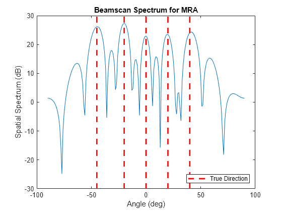
Nested Array
Unfortunately, identifying the architecture for an MRA is not trivial, so such configuration is often not readily available. Recently, nested arrays and coprime arrays have become popular choices for sparse arrays.
A nested array embeds a ULA with small element spacing into another ULA with larger element spacing. Here is an example
Mn = 3;
Nn = 3;
pos_Mn = (0:Mn-1)*d;
pos_Nn = Mn*d:(Mn+1)*d:Nn*(Mn+1)*d;
pos_nested = unique([pos_Mn,pos_Nn]);

helperDisplayArray(pos_nested,'Nested Array');
As you can see, this nested array is formed with a small ULA with half wavelength spacing and then a sparser ULA with 2-wavelength spacing. There are 6 elements in total. For such a nested array, the redundancies can be computed as
pos_nested_idx = round(pos_nested/d);
pos_nested_idx_diff = pos_nested_idx-pos_nested_idx.';
pos_nested_idx_unique = sort(unique(pos_nested_idx_diff(:).'))
pos_nested_idx_unique = 1×23

   -11   -10    -9    -8    -7    -6    -5    -4    -3    -2    -1     0     1     2     3     4     5     6     7     8     9    10    11
Note that we now can construct a 23-element full array. In fact, the degrees of freedom of the full array can be predicted as
N_nested = Mn+Nn;
dof_nested = (N_nested.^2-2)/2+N_nested
dof_nested =
23
Not only a nested array easier to construct than an MRA, but its performance can be easily predicted. For example, there is no closed form solution to construct a 6-element MRA that can be used to reconstruct a full array without any missing elements. The reconstruction process for the nested array is similar to the MRA and is illustrated below.
pos_nested_idx_reconstruct = min(pos_nested_idx_unique):max(pos_nested_idx_unique);
pos_nested_reconstruct = pos_nested_idx_reconstruct*d;

x_nested = sensorsig(pos_nested,N_snap,theta_az,db2pow(-10));
Rxx_nested = x_nested'*x_nested/N_snap;
[~,nested_cov_idx] = ismember(pos_nested_idx_reconstruct(:),pos_nested_idx_diff);
x_full_nested = Rxx_nested(nested_cov_idx);

sv = steervec(pos_nested_reconstruct,ang);
P_full_nested = sv'*x_full_nested;

helperDisplayAngularSpectrum(ang,P_full_nested,theta_az,'Beamscan Spectrum for Nested Array');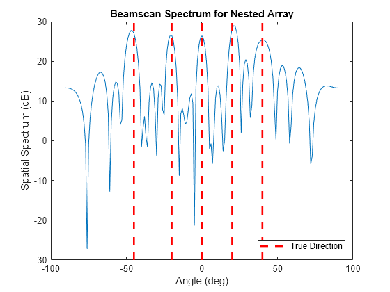
Coprime Arrays
Coprime array is another popular sparse array architecture. The idea of coprime array is to form the array with two subarrays whose element spacings are coprime to each other. The issue with a nested array is that it contains a dense array, making it more prone to mutual coupling effects between array elements. A coprime array is also easy to construct and on average it places elements further apart, thus alleviating the mutual coupling effects.
There are many proposed coprime arrays. This example uses the original coprime array architecture, often termed as the prototype coprime array. A linear prototype coprime array consists of two uniform linear arrays, one with Mc elements and the other Nc elements. Note that Mc and Nc must be coprime. These two arrays share the starting element. In addition, the element spacing of the Mc-element array is Nc*d and the element spacing of the Nc-element array is Mc*d. Assume Mc is 2 and Nc is 3, the sparse array architecture is
Mc = 4;
Nc = 3;
pos_cp_1 = (0:Mc-1)*Nc*d;
pos_cp_2 = (0:Nc-1)*Mc*d;
pos_cp = unique([pos_cp_1 pos_cp_2]);

helperDisplayArray(pos_cp,'Coprime Array');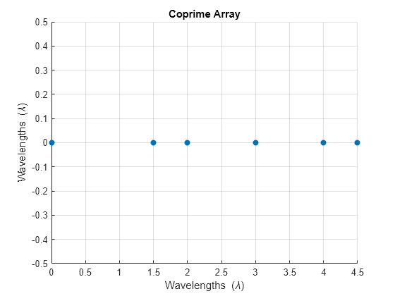
The degrees of freedom of the reconstructed array from a prototype coprime array can be computed as
N_cp = Mc+Nc;
dof_cp = 2*N_cp-1
dof_cp =
13
Let us verify if the degrees of freedom of the reconstructed array matches this.
pos_cp_idx = round(pos_cp/d);
pos_cp_idx_diff = pos_cp_idx-pos_cp_idx.';
pos_cp_idx_unique = sort(unique(pos_cp_idx_diff(:).'))
pos_cp_idx_unique = 1×17

    -9    -8    -6    -5    -4    -3    -2    -1     0     1     2     3     4     5     6     8     9
Notice that even though the reconstructed element lags seem to cover from -9 to 9, there is a gap between lag 6 and 8. Therefore, if we want to reconstruct a fully populated ULA, we can only go from lag -6 to 6, matching the predicted degrees of freedom, 13. The reconstruction process is again similar to other sparse array architectures.
pos_cp_idx_reconstruct = -(dof_cp-1)/2:(dof_cp-1)/2;
pos_cp_reconstruct = pos_cp_idx_reconstruct*d;

x_cp = sensorsig(pos_cp,N_snap,theta_az,db2pow(-10));
Rxx_cp = x_cp'*x_cp/N_snap;
[~,cp_cov_idx] = ismember(pos_cp_idx_reconstruct(:),pos_cp_idx_diff);
x_full_cp = Rxx_cp(cp_cov_idx);

sv = steervec(pos_cp_reconstruct,ang);
P_full_cp = sv'*x_full_cp;

helperDisplayAngularSpectrum(ang,P_full_cp,theta_az,'Beamscan Spectrum for Copime Array');
DOA Estimation Using MUSIC and ESPRIT
Once we obtain the full array, we can just apply any known DOA estimation algorithm to the reconstructed signal measurements. However, it is worth noting that we used many snapshots of a sparse array to derive just one snapshot of the full array. Algorithms like MUSIC and ESPRIT rely on a good estimate of the covariance matrix of the full array, yet we only have one snapshot available. To overcome this issue, we can apply spatial smoothing to the resulting sample covariance matrix to restore enough rank for the DOA estimation, like what we do to handle coherent signal for those algorithms. This certainly reduces the degrees of freedom of the reconstructed array.
Next, use the fully reconstructed array from the coprime array and apply MUSIC algorithm to do the DOA estimation. The illustrated workflow is applicable to both MRA and the nested array.
R_full = x_full_cp*x_full_cp';
% spatial smoothing
ssfactor = (length(x_full_cp)+1)/2;
R_ss = spsmooth(R_full,ssfactor);
[doas_music,spec_music,ang_music] = musicdoa(R_ss,Nsig);

helperDisplayAngularSpectrum(ang_music,spec_music,theta_az,'MUSIC Spectrum for Coprime Array');

fprintf("The estimated directions are: %s",mat2str(sort(doas_music),2))The estimated directions are: [-44 -20 1 20 40]
Applying ESPRIT algorithm follows the same recipe.
doa_esprit = espritdoa(R_ss,Nsig);
fprintf("The estimated directions are: %s",mat2str(sort(doa_esprit),2))
The estimated directions are: [-45 -20 1.3 20 40]
DOA Estimation Using Compressed Sensing
In general, in a DOA estimation scenario, the number of incoming directions is far less than the number of elements. Therefore, the problem is sparse. In addition, trying to identify these directions from a single snapshot also makes the problem underdetermined. Compressive sensing is a family of recently developed techniques that deal with such problems. In this section, we will use orthogonal matching pursuit (OMP) algorithm, which is a basic greedy algorithm in the compressive sensing algorithm family, to perform DOA estimation.
The OMP algorithm relies on a data dictionary. In our case, it consists of steering vectors from all directions. Again, we will use the coprime array architecture to illustrate the workflow.
ang_cs = -90:0.1:90;
sv_dict = steervec(pos_cp_reconstruct,ang_cs);
Then, with a specified maximum sparsity, the OMP algorithm will find a set of steering vectors that best match the given signal. The angles corresponding to those steering vectors are then our DOA estimates.
spec_cs = 1e-3*ones(size(ang_cs)); %-60 dB floor
[p_sp,~,idx_sp] = ompdecomp(x_full_cp,sv_dict,'MaxSparsity',Nsig);
spec_cs(idx_sp) = p_sp;

helperDisplayAngularSpectrum(ang_cs,spec_cs,theta_az,'OMP Spectrum for Comprime Array');

doa_cs = ang_cs(idx_sp);
fprintf("The estimated directions are: %s",mat2str(sort(doa_cs),2))
The estimated directions are: [-44 -20 0.1 20 41]
Summary
In this example, we illustrated several popular sparse array architectures, including MRA, nested arrays, and coprime arrays. We also showed how to reconstruct a full array out of these sparse arrays and then perform either conventional beamscan DOA estimation algorithm or high-resolution DOA estimation algorithms like MUSIC and ESPRIT. We also included a brief discussion on estimating DOAs with compressive sensing using a single snapshot of the array measurements. Sparse arrays allow us to use a smaller number of elements to achieve resolutions, as well as degrees of freedom, of a much larger array. However, a sparse array needs to use many snapshots to reconstruct a single snapshot of the fully reconstructed array. Therefore, this approach may not work very well in rapidly changing environment.
References
[1] Qin, Si, Zhang, Yimin D., and Amin, Moeness G. "Generalized coprime array configurations for direction-of-arrival estimation." IEEE Transactions on Signal Processing 63.6 (2015): 1377-1390.
[2] Vaidyanathan, P. P. and Pal, Piya. "Sparse sensing with coprime arrays." 2010 Conference record of the forty fourth Asilomar conference on signals, systems and computers. IEEE, 2010.
[3] Raza, Ahsan, Liu, Wei, and Shen, Qing. "Thinned Coprime Arrays for DOA Estimation", European Signal Processing Conference, 2017
[4] Pal, Piya and Vaidyanathan, P. P. " Nested Arrays: A Novel Approach to Array Processing with Enhanced Degrees of Freedom" IEEE Transactions on Signal Processing, Vol. 58, No. 8, 2010
[5] Moffet, Alan, "Minimum-Redundancy Linear Arrays" IEEE Transactions on Antennas and Propagation, Vol. AP-16, No. 2, 1968
Helper Functions
helperDisplayArray function
function helperDisplayArray(pos,titlestr)
    scatter(pos,zeros(size(pos)),'o','filled'); grid on
    xlabel('Wavelengths (\lambda)'); ylabel('Wavelengths (\lambda)');
    xlim([min(pos) max(pos)]);
    ylim([-0.5 0.5]);
    title(titlestr);
end
helperDisplayAngularSpectrum function
function helperDisplayAngularSpectrum(ang,spec,trueang,titlestr)
    plot(ang,mag2db(abs(spec)));
    hold on;
    yb = ylim;
    plot(ones(2,1)*trueang,yb(:)*ones(size(trueang)),'r--','LineWidth',2);
    xlabel('Angle (deg)');
    ylabel('Spatial Spectrum (dB)');
    title(titlestr);
    legend('','True Direction','Location','SouthEast');
    hold off;
end