CRLB of Direction of Arrival Estimation

Since R2026a

Introduction

This example demonstrates the computation of the Cramer-Rao Lower Bound (CRLB) of Direction of Arrival (DOA) estimation given a spatial-domain signal. The CRLB provides a theoretical lower bound on the variance of any unbiased DOA estimator. We evaluate the performance of beamscan and MUSIC DOA estimation algorithms by comparing their accuracy against the derived CRLB.

Array Configuration

A 16-element uniform linear array (ULA) with isotropic antennas is constructed, where the inter-element spacing is set to half the wavelength. The array receives narrowband signals with a carrier frequency of 1 GHz. Data is collected over 64 independent snapshots, which may be obtained at different time instants to ensure statistical independence.

rng('default')
N = 16;
Nsnapshots = 64;
fc = 1e9;
lambda = freq2wavelen(fc);
antenna = phased.IsotropicAntennaElement;
array = phased.ULA('Element',antenna,'NumElements',N,'ElementSpacing',lambda/2);

The received signal originates from a source at 9° azimuth and is corrupted by additive white Gaussian noise (AWGN) with a noise power of 1 Watt. We evaluate the DOA estimation accuracy across varying signal-to-noise ratios (SNRs), defined as the ratio of the received signal power to the noise power.

powdb = -20:5:5;
Nsnr = length(powdb);
amp = db2mag(powdb);
doa = 9;
phase = pi/4;
npow = 1;

Signal Model

The received signal at the ULA for a single source is modeled as:

$s (p) = A \exp (j (π \sin (θ) n + ϕ)), n = [0, 1, \dots, N - 1]^{T},$

where $N$ is the number of ULA elements, and $p = [A, θ, ϕ, σ^{2}]^{T}$ is the vector of unknown parameters:

$A$ : signal amplitude,
$θ$ : DOA (azimuth angle),
$ϕ$ : phase offset,
$σ^{2}$ : noise power.

The noise is additive white Gaussian (AWGN) with spatial covariance matrix:

$R = σ^{2} I_{N},$

where $I_{N}$ is the $N \times N$ identity matrix.

The signal model is implemented as an anonymous function.

sig = @(p) p(1) * exp(1j * (pi * sind(p(2)) * (0:N-1)' + p(3)));

The noise model is similarly defined.

ncov = @(p) p(4);

CRLB Computation for DOA Estimation

The CRLB matrix for $p = [A, θ, ϕ, σ^{2}]^{T}$ is computed numerically under varying SNR conditions. As the DOA is the second parameter in $p$ , the DOA CRLB (variance lower bound for $θ$ ) is extracted as the second diagonal entry of the CRLB matrix.

crlb_doa = zeros(1,Nsnr);
for snridx = 1:Nsnr
    param = [amp(snridx), doa, phase, npow]';
    crlb_numerical = crlb(sig, ncov, param);
    crlb_doa(snridx) = crlb_numerical(2,2);
end

The CRLB is scaled by the number of snapshots to account for processing gain.

crlb_doa = crlb_doa/Nsnapshots;

Monte Carlo Simulation for DOA Estimation

Configure the beamscan and MUSIC estimators with a scan range of −15° to 15° (0.01° resolution).

scanang = -15:0.01:15;
beamscan = phased.BeamscanEstimator('SensorArray',array,'ScanAngles',scanang, ...
    'OperatingFrequency',fc,'DOAOutputPort',true,'NumSignals',1);
music = phased.MUSICEstimator('SensorArray',array,'ScanAngles',scanang,...
    'OperatingFrequency',fc,'DOAOutputPort',true,...
    'NumSignalsSource','Property','NumSignals',1);

For each SNR, simulate 1000 trials of beamscan and MUSIC estimation.

Ntrials = 1e3;
beamscan_doa_est = zeros(Ntrials,Nsnr);
music_doa_est = zeros(Ntrials,Nsnr);
for snridx = 1:Nsnr
    sig = amp(snridx) * exp(1j*(pi * sind(doa) * (0:N-1) + phase)); 
    noise = (randn(Nsnapshots*Ntrials,N) + 1i*randn(Nsnapshots*Ntrials,N))*chol(npow/2,'upper'); 
    for trialIdx = 1:Ntrials
        x = sig + noise((trialIdx-1)*Nsnapshots+1:trialIdx*Nsnapshots,:);
        [~,beamscan_doas] = beamscan(x);
        beamscan_doa_est(trialIdx,snridx) = beamscan_doas;
        [~,music_doas] = music(x);
        music_doa_est(trialIdx,snridx) = music_doas;
    end
end

Compute the Mean Squared Error (MSE) for both estimators.

beamscan_doa_est_mse = rmse(beamscan_doa_est,doa,1,"omitnan").^2;
music_doa_est_mse = rmse(music_doa_est,doa,1,"omitnan").^2;

Compare the MSE of the beamscan and MUSIC DOA estimators against the theoretical CRLB across varying SNR levels.

figure
plot(powdb,crlb_doa)
hold on;
plot(powdb,beamscan_doa_est_mse,'-*')
plot(powdb,music_doa_est_mse,'-o')
xlabel('SNR (dB)')
ylabel('MSE (degrees squared)')
yscale("log")
title('DOA Estimation MSE')
legend('CRLB','Beamscan','MUSIC')
grid on; hold off;

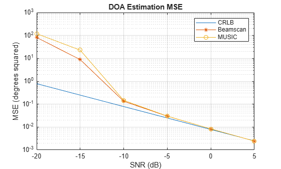
Figure contains an axes object. The axes object with title DOA Estimation MSE, xlabel SNR (dB), ylabel MSE (degrees squared) contains 3 objects of type line. These objects represent CRLB, Beamscan, MUSIC.

The plot demonstrates that in the high-SNR regime, both the beamscan and MUSIC estimators achieve MSE values that converge to the CRLB, indicating their asymptotic efficiency.