Simulate Battery Discharge-Rest-CC-CV Charge Cycle

R2026b

This example shows how to set up a pseudo-2D (P2D) battery model and simulate a full discharge-rest-charge cycle with a constant-current constant-voltage (CC-CV) charging protocol. The model uses parameters for a 12 Ah nickel cobalt aluminum (NCA) pouch lithium-ion cell from Jin et al. [1].

Define Active Materials

Create the anode and cathode active materials by specifying particle geometry, concentration limits, diffusion coefficients, reaction kinetics, and open-circuit potential (OCP) functions.

The OCP functions are polynomial fits from the parameterization study. The stoichiometric limits define the range of lithium intercalation used during cycling: the first value is the stoichiometry at 0% SOC and the second is the stoichiometry at 100% SOC.

anodeMaterial = batteryActiveMaterial( ...
    ParticleRadius=0.834e-6, ...
    MaximumSolidConcentration=16.1e3, ...
    VolumeFraction=0.58, ...
    DiffusionCoefficient=2e-14, ...
    ReactionRate=4.5229e-11, ...
    OpenCircuitPotential=@anodeOCP, ...
    StoichiometricLimits=[0.126 0.676]);

cathodeMaterial = batteryActiveMaterial( ...
    ParticleRadius=0.834e-6, ...
    MaximumSolidConcentration=23.9e3, ...
    VolumeFraction=0.5, ...
    DiffusionCoefficient=8.38e-16, ...
    ReactionRate=2.0976e-11, ...
    OpenCircuitPotential=@cathodeOCP, ...
    StoichiometricLimits=[0.442 0.936]);

Define Electrodes and Separator

Create the anode and cathode electrodes with thickness, porosity, Bruggeman coefficient, and electrical conductivity. The Bruggeman coefficient accounts for the tortuous path ions take through the porous electrode.

anodeElectrode = batteryElectrode( ...
    Thickness=5e-5, ...
    Porosity=0.21, ...
    BruggemanCoefficient=1.5, ...
    ElectricalConductivity=1000, ...
    ActiveMaterial=anodeMaterial);

cathodeElectrode = batteryElectrode( ...
    Thickness=3.64e-5, ...
    Porosity=0.25, ...
    BruggemanCoefficient=1.5, ...
    ElectricalConductivity=0.002, ...
    ActiveMaterial=cathodeMaterial);

separator = batterySeparator( ...
    Thickness=2.54e-5, ...
    Porosity=0.5, ...
    BruggemanCoefficient=1.5);

Define Electrolyte

Create the electrolyte with a constant diffusion coefficient, ionic conductivity, and transference number. In this parameterization, these properties are not concentration-dependent.

electrolyte = batteryElectrolyte( ...
    DiffusionCoefficient=1.66e-11, ...
    IonicConductivity=0.29, ...
    TransferenceNumber=0.35);

Set Initial Conditions and Assemble the Model

Define the initial electrolyte concentration, state of charge (SOC), and temperature. Assemble all components into a P2D battery model.

ic = batteryInitialConditions( ...
    ElectrolyteConcentration=1200, ...
    StateOfCharge=1, ...
    Temperature=298.15);

model = batteryP2DModel( ...
    Anode=anodeElectrode, ...
    Separator=separator, ...
    Cathode=cathodeElectrode, ...
    Electrolyte=electrolyte, ...
    InitialConditions=ic);

Define Cycling Steps

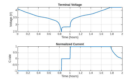
Set up a four-step cycling protocol:

• Discharge: 1C constant current until voltage reaches 2.5 V

• Rest: No current for 600 seconds

• CC Charge: 1C constant current until voltage reaches 4.2 V

• CV Charge: Hold voltage at 4.2 V until current drops to C/20

discharge = batteryCyclingStep;
discharge.NormalizedCurrent = -1;
discharge.CutoffVoltageLower = 2.5;
discharge.OutputTimeStep = 10;

rest = batteryCyclingStep;
rest.NormalizedCurrent = 0;
rest.CutoffTime = 600;
rest.OutputTimeStep = 10;

ccCharge = batteryCyclingStep;
ccCharge.NormalizedCurrent = 1;
ccCharge.CutoffVoltageUpper = 4.2;
ccCharge.OutputTimeStep = 10;

cvCharge = batteryCyclingStep;
cvCharge.HoldVoltage = 4.2;
cvCharge.CutoffNormalizedCurrent = 0.05;
cvCharge.OutputTimeStep = 10;

model.CyclingStep = [discharge, rest, ccCharge, cvCharge];

Solve the Model

Run the simulation for the complete cycling sequence.

R = solve(model);

Performing cycling step: 1 of 4
Performing cycling step: 2 of 4
Performing cycling step: 3 of 4
Performing cycling step: 4 of 4

Plot Results

Plot a summary of all quantities of interest from the simulation results.

plotSummary(R)

Visualize the terminal voltage and normalized current (C-rate) over time.

figure
tiledlayout(2,1)

nexttile
plot(R.SolutionTimes/3600, R.TerminalVoltage, LineWidth=1.5)
xlabel("Time (hours)")
ylabel("Voltage (V)")
title("Terminal Voltage")
grid on

nexttile
plot(R.SolutionTimes/3600, R.NormalizedCurrent, LineWidth=1.5)
xlabel("Time (hours)")
ylabel("C-rate")
title("Normalized Current")
grid on

References

[1] Jin N, Danilov DL, Van den Hof PMJ, Donkers MCF. Parameter estimation of an electrochemistry-based lithium-ion battery model using a two-step procedure and a parameter sensitivity analysis. Int J Energy Res. 2018;42:2417-2430. https://doi.org/10.1002/er.4022

Local Functions

Open-circuit potential functions for the anode and cathode, defined as polynomial fits from [1].

function Un = anodeOCP(theta)
y = (theta - 0.126) ./ (0.676 - 0.126);
gamma = [0.0004, -0.0145, 0.1115, -0.6830, 0.8020, ...
         -0.3611, 0.1115, 0.0171, 0.1115, 0.0171];
Un = gamma(1).*y.^(-1) ...
   + gamma(2).*y.^(-0.5) ...
   + gamma(3) ...
   + gamma(4).*y.^(0.5) ...
   + gamma(5).*y.^(1.0) ...
   + gamma(6).*y.^(1.5) ...
   + gamma(7).*exp(gamma(8).*y) ...
   + gamma(9).*exp(gamma(10).*y);
end

function Up = cathodeOCP(theta)
y = (0.936 - theta) ./ (0.936 - 0.442);
gamma = [-2.2049e3, 11.2250, -112.9966, 647.4250, -2.083e3, ...
          3.7868e3, -3.6869e3, 1.5388e3, 2.2079e3, -0.0464];
Up = gamma(1) ...
   + gamma(2).*y.^1 ...
   + gamma(3).*y.^2 ...
   + gamma(4).*y.^3 ...
   + gamma(5).*y.^4 ...
   + gamma(6).*y.^5 ...
   + gamma(7).*y.^6 ...
   + gamma(8).*y.^7 ...
   + gamma(9).*exp(gamma(10).*y.^10);
end