Heat Transfer in Block with Cavity

This example shows how to solve for the heat distribution in a block with cavity.

Consider a block containing a rectangular crack or cavity. The left side of the block is heated to 100 degrees centigrade. At the right side of the block, heat flows from the block to the surrounding air at a constant rate, for example $$-10W/m^2$$. All the other boundaries are insulated. The temperature in the block at the starting time $$t_0=0$$ is 0 degrees. The goal is to model the heat distribution during the first five seconds.

Create Thermal Analysis Model

The first step in solving a heat transfer problem is to create a thermal analysis model. This is a container that holds the geometry, thermal material properties, internal heat sources, temperature on the boundaries, heat fluxes through the boundaries, mesh, and initial conditions.

thermalmodel = createpde("thermal","transient");

Import Geometry

Add the block geometry to the thermal model by using the geometryFromEdges function. The geometry description file for this problem is called crackg.m.

geometryFromEdges(thermalmodel,@crackg);

Plot the geometry, displaying edge labels.

pdegplot(thermalmodel,"EdgeLabels","on")
ylim([-1,1])
axis equal

Specify Thermal Properties of Material

Specify the thermal conductivity, mass density, and specific heat of the material.

thermalProperties(thermalmodel,"ThermalConductivity",1,...
                               "MassDensity",1,...
                               "SpecificHeat",1);

Apply Boundary Conditions

Specify the temperature on the left edge as 100, and constant heat flow to the exterior through the right edge as -10. The toolbox uses the default insulating boundary condition for all other boundaries.

thermalBC(thermalmodel,"Edge",6,"Temperature",100);
thermalBC(thermalmodel,"Edge",1,"HeatFlux",-10);

Set Initial Conditions

Set an initial value of 0 for the temperature.

thermalIC(thermalmodel,0);

Generate Mesh

Create and plot a mesh.

generateMesh(thermalmodel);
figure
pdemesh(thermalmodel)
title("Mesh with Quadratic Triangular Elements")

Specify Solution Times

Set solution times to be 0 to 5 seconds in steps of 1/2.

tlist = 0:0.5:5;

Calculate Solution

Use the solve function to calculate the solution.

thermalresults = solve(thermalmodel,tlist)

thermalresults = 
  TransientThermalResults with properties:

      Temperature: [1320x11 double]
    SolutionTimes: [0 0.5000 1 1.5000 2 2.5000 3 3.5000 4 4.5000 5]
       XGradients: [1320x11 double]
       YGradients: [1320x11 double]
       ZGradients: []
             Mesh: [1x1 FEMesh]

Evaluate Heat Flux

Compute the heat flux density.

[qx,qy] = evaluateHeatFlux(thermalresults);

Plot Temperature Distribution and Heat Flux

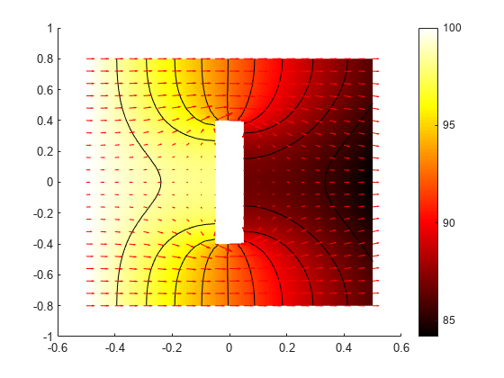
Plot the solution at the final time step, t = 5.0 seconds, with isothermal lines using a contour plot, and plot the heat flux vector field using arrows.

pdeplot(thermalmodel,"XYData",thermalresults.Temperature(:,end), ...
                     "Contour","on",...
                     "FlowData",[qx(:,end),qy(:,end)], ...
                     "ColorMap","hot")

×

Open Example

You have a modified version of this example. Do you want to open this example with your edits?

No, overwrite the modified version Yes