Get Started with Time Series Forecasting
This example shows how to create a simple long short-term memory (LSTM) network to forecast time series data using the Deep Network Designer app.
An LSTM network is a recurrent neural network (RNN) that processes input data by looping over time steps and updating the RNN state. The RNN state contains information remembered over all previous time steps. You can use an LSTM neural network to forecast subsequent values of a time series or sequence using previous time steps as input.

Load Sequence Data
Load the example data from WaveformData. To access this data, open the example as a live script. The Waveform data set contains synthetically generated waveforms of varying lengths with three channels. The example trains an LSTM neural network to forecast future values of the waveforms given the values from previous time steps.
load WaveformDataVisualize some of the sequences.
idx = 1;
numChannels = size(data{idx},2);

figure
stackedplot(data{idx},DisplayLabels="Channel " + (1:numChannels))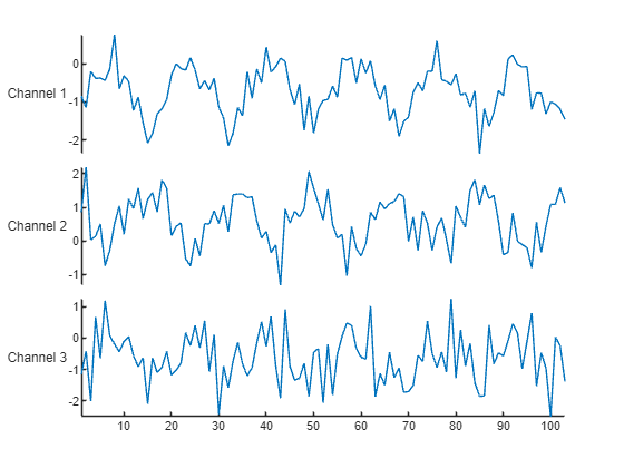
For this example, use the helper function prepareForecastingData, attached to this example as a supporting file, to prepare the data for training. This function prepares the data using these steps:
To forecast the values of future time steps of a sequence, specify the targets as the training sequences with values shifted by one time step. At each time step of the input sequence, the LSTM neural network learns to predict the value of the next time step. Do not include the final time step in the training sequences.
Partition the data into a training set containing 90% of the data and a test set containing 10% of the data.
[XTrain,TTrain,XTest,TTest] = prepareForecastingData(data,[0.9 0.1]);
For a better fit and to prevent the training from diverging, you can normalize the predictors and targets so that the channels have zero mean and unit variance. When you make predictions, you must also normalize the test data using the same statistics as the training data. For more information, see Build Time Series Forecasting Network Using Deep Network Designer.
Define Network Architecture
To build the network, open the Deep Network Designer app.
deepNetworkDesigner
To create a sequence network, in the Sequence Networks section, pause on Sequence to Sequence and click Open.
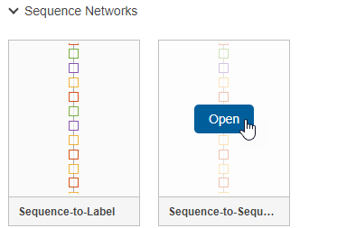
Doing so opens a prebuilt network suitable for sequence classification problems. You can convert the classification network into a regression network by editing the final layers.
First, delete the softmax layer.
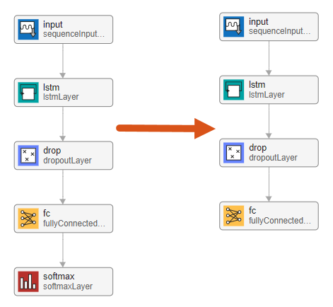
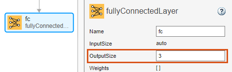
Next, adjust the properties of the layers so that they are suitable for the Waveform data set. Because the aim is to forecast future data points in a time series, the output size must be the same as the input size. In this example, the input data has three input channels so, the network output must also have three output channels.
Select the sequence input layer input and set InputSize to 3.

Select the fully connected layer fc and set OutputSize to 3.
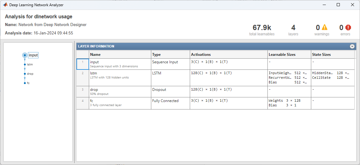
To check that the network is ready for training, click Analyze. The Deep Learning Network Analyzer reports zero errors or warnings, so the network is ready for training. To export the network, click Export. The app saves the network in the variable net_1.
Specify Training Options
Specify the training options. Choosing among the options requires empirical analysis. To explore different training option configurations by running experiments, you can use the Experiment Manager app. Because the recurrent layers process sequence data one time step at a time, any padding in the final time steps can negatively influence the layer output. Pad or truncate sequence data on the left by setting the SequencePaddingDirection option to "left".
options = trainingOptions("adam", ...
    MaxEpochs=300, ...
    SequencePaddingDirection="left", ...
    Shuffle="every-epoch", ...
    Plots="training-progress", ...
    Verbose=false);
Train Neural Network
Train the neural network using the trainnet function. Because the aim is regression, use mean squared error (MSE) loss.
net = trainnet(XTrain,TTrain,net_1,"mse",options);
Forecast Future Time Steps
Closed loop forecasting predicts subsequent time steps in a sequence by using the previous predictions as input.
Select the first test observation. Initialize the RNN state by resetting the state using the resetState function. Then use the predict function to make an initial prediction Z. Update the RNN state using all time steps of the input data.
X = XTest{1};
T = TTest{1};

net = resetState(net);
offset = size(X,1);
[Z,state] = predict(net,X(1:offset,:));
net.State = state;
To forecast further predictions, loop over time steps and make predictions using the predict function and the value predicted for the previous time step. After each prediction, update the RNN state. Forecast the next 200 time steps by iteratively passing the previous predicted value to the RNN. Because the RNN does not require the input data to make any further predictions, you can specify any number of time steps to forecast. The last time step of the initial prediction is the first forecasted time step.
numPredictionTimeSteps = 200;
Y = zeros(numPredictionTimeSteps,numChannels);
Y(1,:) = Z(end,:);

for t = 2:numPredictionTimeSteps
    [Y(t,:),state] = predict(net,Y(t-1,:));
    net.State = state;
end

numTimeSteps = offset + numPredictionTimeSteps;
Compare the predictions with the input values.
figure
l = tiledlayout(numChannels,1);
title(l,"Time Series Forecasting")

for i = 1:numChannels
    nexttile
    plot(X(1:offset,i))
    hold on
    plot(offset+1:numTimeSteps,Y(:,i),"--")
    ylabel("Channel " + i)
end

xlabel("Time Step")
legend(["Input" "Forecasted"])
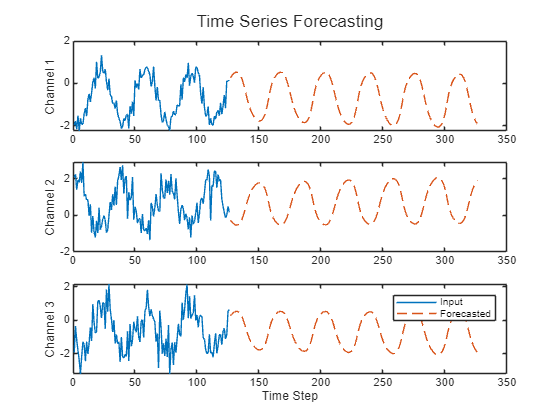
This method of prediction is called closed-loop forecasting. For more information about time series forecasting and performing open-loop forecasting, see Time Series Forecasting Using Deep Learning.
See Also
dlnetwork | trainingOptions | trainnet | scores2label | Deep Network
Designer
Related Topics
You can also select a web site from the following list:
Americas
- América Latina (Español)
- Canada (English)
- United States (English)
Europe
- Belgium (English)
- Denmark (English)
- Deutschland (Deutsch)
- España (Español)
- Finland (English)
- France (Français)
- Ireland (English)
- Italia (Italiano)
- Luxembourg (English)
- Netherlands (English)
- Norway (English)
- Österreich (Deutsch)
- Portugal (English)
- Sweden (English)
- Switzerland
- United Kingdom (English)