Resolver Decoder
Compute motor mechanical position and speed and sine and cosine values of motor electrical position
Libraries:
Motor Control Blockset /
Sensor Decoders
Description
The Resolver Decoder block computes the following for a resolver connected to the motor shaft:
Mechanical angular position of motor
Sine and cosine values of electrical angular position of motor
Mechanical speed of motor
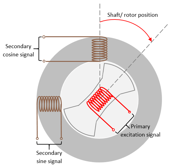
A resolver uses a primary excitation input signal to generate the modulated secondary sine and cosine waveforms, which are then sampled by the ADC. The resolver utilizes one winding to two winding transformations. The sine and cosine modulation occurs in the secondary windings because of the design and construction of these windings, which places them at positions that are 90 degrees apart.

For more details about the algorithm used by the block, see Algorithm.
Examples
Monitor Resolver Using Serial Communication
Use the resolver sensor to measure the rotor position. The resolver consists of two stator (secondary) windings placed orthogonally around the resolver rotor (primary) winding. After you mount the resolver sensor over a PMSM, the resolver rotor winding rotates with the shaft of the running motor. Meanwhile, the controller provides a fixed-frequency excitation signal (alternating sinusoidal or square pulse) to the primary winding.
Ports
Input
Output
Parameters
Algorithms
The block uses the correctly sampled and normalized version of the secondary sine and cosine waveforms to demodulate the sine and cosine signals using which it determines the electrical position of the resolver. It converts this position into its mechanical equivalent according to the number of pole pairs available in the resolver. The resulting value indicates the mechanical position of the motor.
The block also uses the demodulated sine and cosine signals (sine and cosine of resolver electrical angle) to compute the motor speed as well as the sine and cosine values of the motor electrical position.
When you use the sinusoidal excitation method, the block expects secondary sine and cosine resolver signals sampled, by default, at the rate of 16 samples per excitation signal cycle, as shown in the diagram. The block can also add a phase delay to the sampled sine and cosine signals with respect to the excitation signal.
When using sinusoidal excitation, the block does not normalize the modulated sine and cosine resolver output automatically. You need to normalize these modulated waveforms (within the range of [-1,1] and centred at 0) before inputting them to the block.
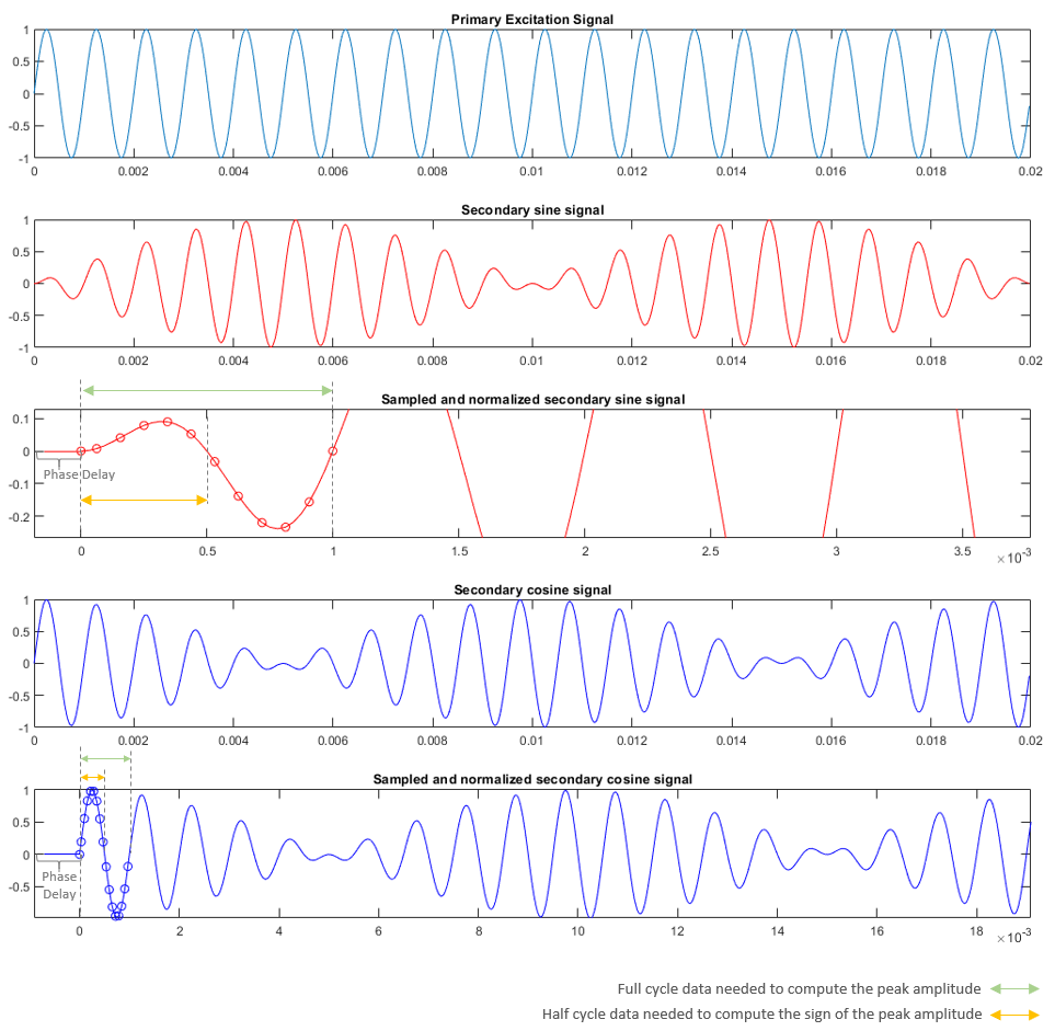
The block then demodulates the sampled signal. It computes the average and peak amplitude values and the sign of the peak amplitude of a signal cycle as
and
where:
is the average amplitude value of a signal cycle.
is the number of samples per excitation cycle.
is the peak amplitude value of a signal cycle.
The block computes the electrical angular position of the resolver as
where:
is the of the secondary sine signal.
is the of the secondary cosine signal.
is the electrical angular position of the resolver.
This enables the block to demodulate and extract the sine and cosine envelopes. The block uses these demodulated envelop signals to compute the block outputs.
When using the square pulse excitation method, the block expects the secondary sine and cosine signals sampled at the rate of one sample every pulse as shown below.
If you select the Enable input normalization parameter, then after receiving the discrete-time sampled waveform, the block automatically normalizes the waveform (within the range of [-1,1] and centred at 0). To perform normalization within the block, ensure that both input signals have equal peak magnitudes.
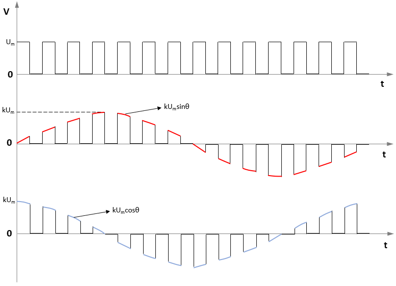
The block then demodulates the sine and cosine signals and uses the demodulated signals to compute the block outputs.
When using either sinusoidal or square-pulse excitation, the block uses the demodulated waveforms to compute the electrical position of the resolver. This resolver position can vary using either a positive ramp (for clockwise rotation) or a negative ramp (for counterclockwise rotation).
To correctly detect the wrap-around (from 0 PU to 1 PU or from 1 PU to 0 PU), the block measures the difference between the two consecutive samples. Because the input signal frequency is always less than half of the sampling frequency, a difference less than –0.5 PU indicates a positive ramp whereas a difference that is less than +0.5 PU indicates a negative ramp.

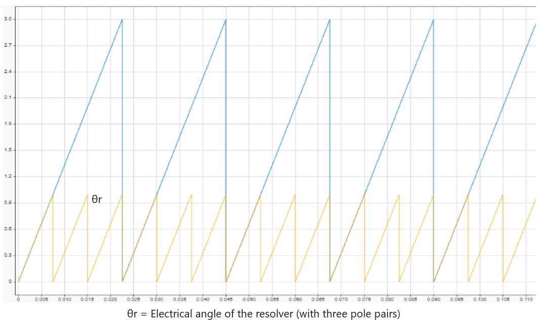
After identifying the resolver electrical position direction, the block uses the number of resolver pole pairs to compute the mechanical position of the resolver (and the motor) by extrapolating the ramp signal.
For example, for a three-pole pair resolver, the block extrapolates the ramp to achieve a magnitude that is three times the original magnitude. It then divides the value by 3 to obtain the resolver mechanical position as shown in these plots.
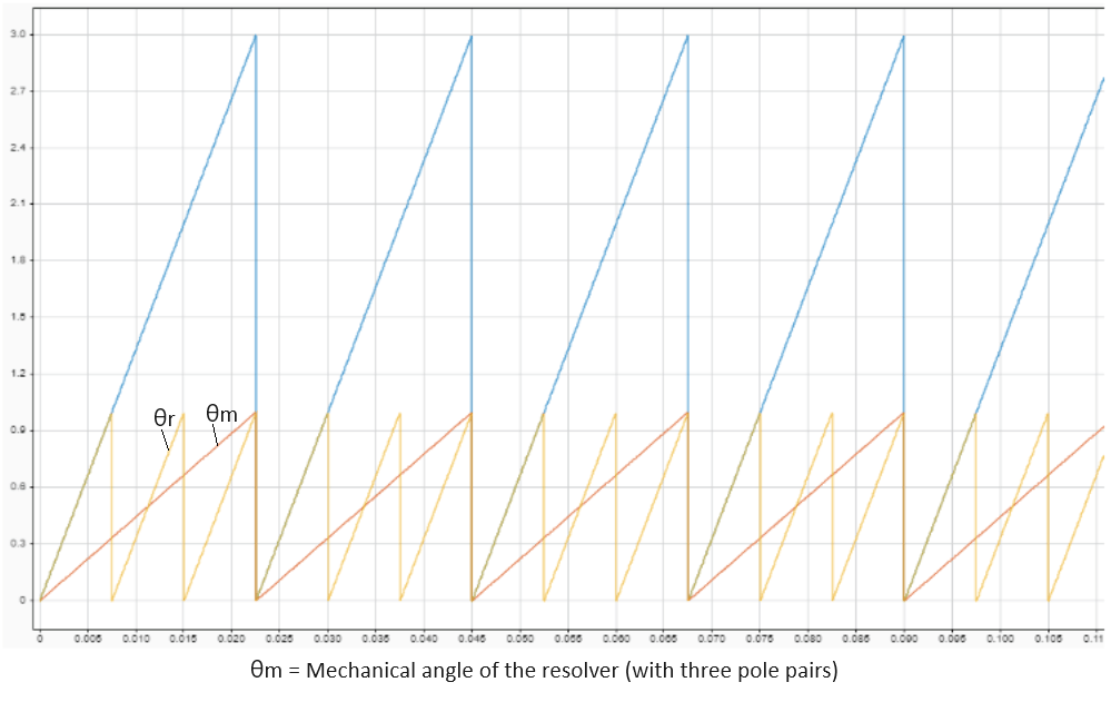
This section shows how the block uses arithmetic operations to compute mechanical position of the motor. Alternatively, the block can also compute the mechanical position using an algorithm based on phase-locked loop (PLL). For details about the PLL-based computation method, see PLL with Feed Forward.
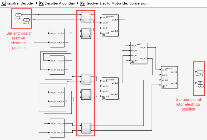
When using either sinusoidal or square-pulse excitation, the block generates the demodulated sine and cosine waveforms (sine and cosine of resolver electrical position). From these demodulated waveforms, the block computes the sine and cosine of the motor electrical position using an arithmetic computation according to the ratio of the motor and resolver pole pairs. To accommodate for different possible ratios, the block utilizes unit blocks, which in turn use a structure based on the generic binary coded decimal (BCD).
For example, if the ratio of motor and resolver pole pairs (n) is 5, the following image shows the BCD-based algorithm that eventually generates the sine and cosine of the motor electrical position.
Therefore, n = number of motor pole pairs/ number of resolver pole pairs = 5.
BCD code for n = 5 is [0 0 1 0
1] or [24 23
22 21
20]. The block configures the algorithm for this
sequence as shown below.
The block supports values of n (integers) ranging from 1 to 31.
Note
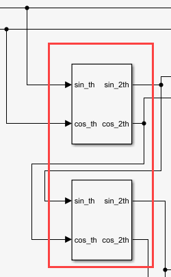
The block optimizes the computation according to the ratio n. For
example, if n = 5, the block only computes
sin_2th and cos_2th twice by utilizing the
following two subsystems only.
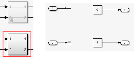
Similarly, whenever a switch does not bypass the signals, it terminates them as shown in the diagram to ensure minimal and optimized code generation.
This section shows how the block uses arithmetic operations to compute the sine and cosine equivalents of electrical motor position. Alternatively, the block can also compute the sine and cos equivalents of electrical position using an algorithm based on phase-locked loop (PLL). For details about the PLL-based computation method, see PLL with Feed Forward.
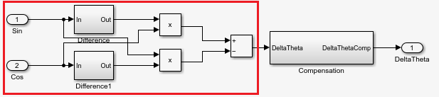
When using either sinusoidal or square-pulse excitation, the block generates the demodulated sine and cosine waveforms (sine and cosine of resolver electrical position). From these waveforms, the block computes the motor mechanical speed using the algorithm described here.
First, the block computes the difference between the two samples of these discrete time sampled signals and adds them.
In the ideal scenario, when using continuous time signals:
Where, ωr is constant with respect to time.
Because we use discrete time sampled signals:
If ωxTs is very small, then
sinωrTs approximately
equals ωrTs. This is
speed x time, therefore, this term indicates position difference for a
sample duration Δθ.
To obtain a more accurate speed, we use the Taylor series expansion of sin-1 to add the following compensation of .
Because the error is negligible, the preceding ωr value can be considered as accurate. Therefore, we can state:
where, Pr is the number of pole pairs of resolver.
The block multiplies the gain of separately to avoid data overflow when using a fixed-point data type.
Here, is the approximate compensation that the block applies to the computed speed as shown in the diagram to obtain a more accurate version of the actual mechanical speed.

where:
g is the speed conversion factor.
θ is the electrical position of the resolver.
ωr is the electrical speed of the resolver.
Δθ is the resolver electrical position difference per sample.
ω is the mechanical speed of the resolver (or motor).
Ts is the sampling time of the sine and cosine envelop signals.
Note
All block inputs should have identical amplitude and data types (either signed fixed or floating point).
This section shows how the block uses arithmetic operations to compute motor speed. Alternatively, the block can also compute the motor speed using an algorithm based on phase-locked loop (PLL). For details about the PLL-based computation method, see PLL with Feed Forward.
References
[1] The block's capability of resolver excitation using square-pulse carrier frequency is based on the collaboration (IITD/FT/03/2038/2020) between The MathWorks, Inc. and Indian Institute of Technology (IIT), Delhi - with inputs from Prof. Amit Kumar Jain (Faculty Consultant-Incharge, EE, IIT Delhi) and Apurva Verma (PhD student, IIT Delhi).
Extended Capabilities
Version History
Introduced in R2020a