SynRM Constraint Curves and Their Application

Open Live Script

This example uses Motor Control Blockset™ to utilize the motor constraint curves to determine the operating currents and use lookup tables of these currents in simulation or deployment environments. The example uses the PMSM constraint curves described in the PMSM Drive Characteristics and Constraint Curves page.

Synchronous reluctance motor (SynRM) or permanent magnet-assisted synchronous reluctance motor (PMaSynRM) have two different definitions of the d-q axis notation. One of them is identical to that of a permanent magnet synchronous motor (PMSM). The alternate notation is a 90 degrees electically rotated notation, which is different from the notation of a PMSM.

In a standard PMSM, the d-axis of the dq rotating reference frame is oriented towards the direction of the magnetic field from the rotor to stator. Usually, this direction aligns with the middle of the hypothetical rotor magnet, with the north facing the stator. We can assume the same for a PMaSynRM. When using the first notation for a SynRM, the d-axis is used as the direction which aligns with the symmetric center of the rotor slots, where the magnets would have been located if the motor were of the PMaSynRM type. This representation makes the constraint curves and the characteristic equations identical to that of a PMSM.

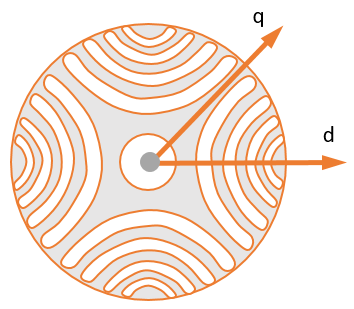
Figure 1: Representation of d- and q-axes for a SynRM, which is identical to that of a PMSM.

When using the alternate notation, the d-axis is defined as the direction of maximum flux transfer. For a SynRM, the d-axis lies between the rotor slots. For a PMaSynRM, the maximum flux transfer from the rotor to the stator happens in the same direction because the magnet is designed to be weaker.

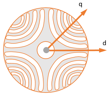
Figure 2: Representation of d- and q-axes for a SynRM, which is different from that of a PMSM.

The PMSM Constraint Curves and Their Application example explains the constraint curves of a PMSM. The five curves (current limit circle, constant torque curve, MTPA curve, voltage limit curve, and MTPV curve) represent the constraints and characteristics of a motor system.

When using an axis notation that is identical to that of a PMSM, the constraint curves are drawn in the second quadrant of the id-iq plane. When using an axis notation that is different from that of a PMSM, the constraint curves are drawn in first quadrant of the id-iq plane.

Required MathWorks Products

Motor Control Blockset
Simulink®

Constraint Curves of PMSM

The constraint curves represent the operational constraints of PMSM control. Each curve corresponds to either a constraint or a characteristic behavior.

Use the following code to re-create figure 3.

pmsm=mcb_SetPMSMMotorParameters('Teknic2310P');
pmsm.Rs=0.01;
pmsm.FluxPM=0.001;
pmsm.Lq=pmsm.Ld*2;
inverter=mcb_SetInverterParameters('BoostXL-DRV8305');
mcbPMSMCharacteristics(pmsm,inverter,speed=10000,torque=0.05);
xlim([-25 +15]);
ylim([-10 +20]);

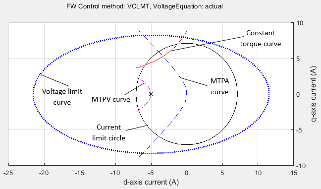
Figure 3: Representation of constraint curves of a PMSM.

Use the following code to re-create figure 4.

motor=mcb_SetPMSMMotorParameters('Teknic2310P');
motor.Rs=1;
motor.FluxPM=0;
motor.Lq=motor.Ld*5;
inverter=mcb_SetInverterParameters('BoostXL-DRV8305');
mcbPMSMCharacteristics(motor,inverter,speed=5500,torque=0.1);
xlim([-17 +17]);
ylim([-8 +8]);

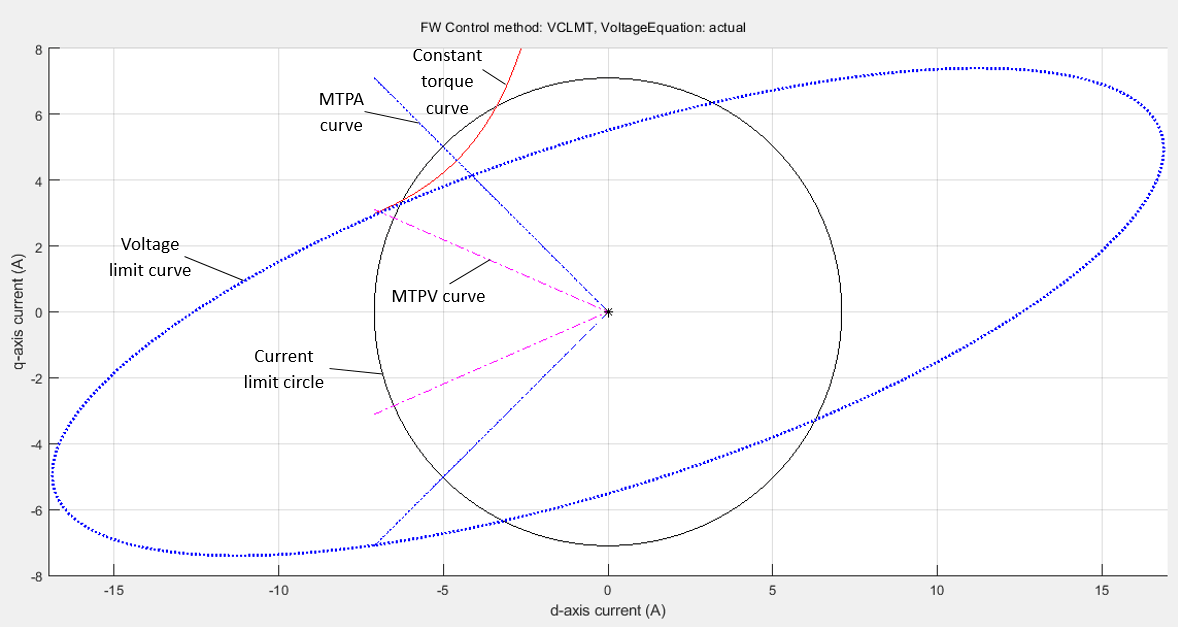
Figure 4: Representation of constraint curves of SynRM when the axis notation is identical to that of a PMSM.

Use the following code to re-create figure 5.

motor=mcb_SetPMSMMotorParameters('Teknic2310P');
motor.Rs=1;
motor.FluxPM=0;
motor.Lq=motor.Ld*5;
inverter=mcb_SetInverterParameters('BoostXL-DRV8305');
mcbPMSMCharacteristics(motor,inverter,speed=5500,torque=0.1,changeDQAxes=1);
xlim([-10 +10]);
ylim([-18 +18]);

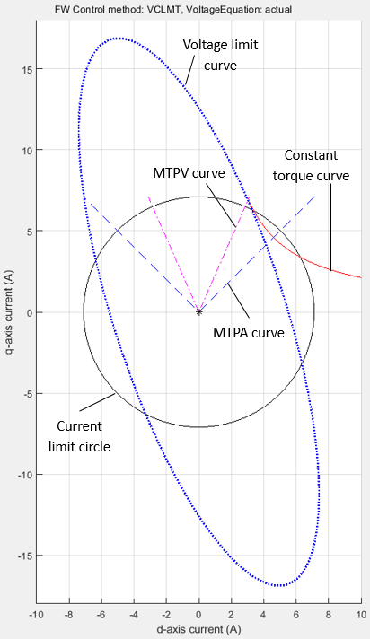
Figure 5: Representation of constraint curves of SynRM when the axis notation is different from that of a PMSM.

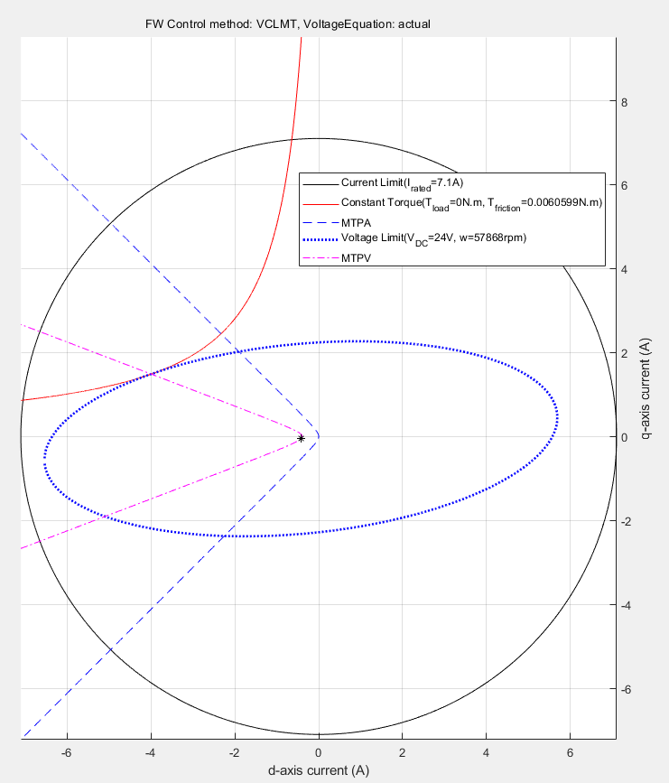
Figure 6: Representation of constraint curves of a PMaSynRM when the axis notation is identical to that of a PMSM.

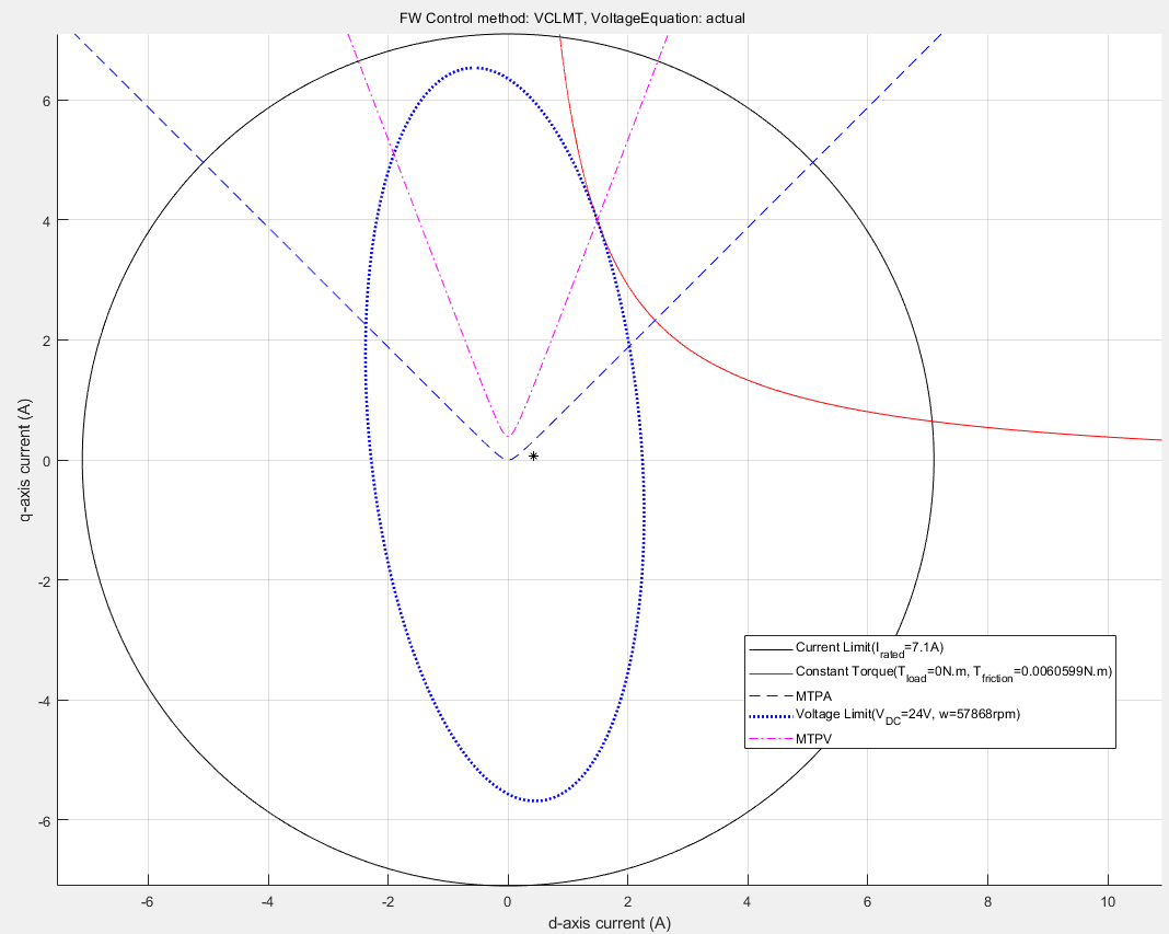
Figure 7: Represenation of constraint curves of a PMaSynRM when the axis notation is different from that of a PMSM.

The d-q Frame of Reference

The d-q frame of reference is a rotating frame of reference that rotates along with the rotor. Unlike the stationary frame of reference, the d-q frame of reference simplifies the representation of the electrical quantities of a motor, such as voltages and currents.

You can measure the motor phase currents ia, ib, and ic and transform them into d-q reference frame currents (id, iq) using the rotor position. For a balanced three-phase system, you can assume that the zero-sequence current is equal to zero. For more details about the Clarke and Park transformations, see Clarke and Park Transforms - MATLAB & Simulink (mathworks.com).

The d-q Current Space

This is the imaginary frame of reference with the d-axis current represented on the x-axis and the q-axis current represented on the y-axis.

You can plot the limits and characteristics of a given PMSM (when represented in terms of id and iq) in the d-q current space.

Explanation for each of the curves is provided in the other example titled PMSM Constraint Curves and Their Application. The curves hold the same meaning irrespective of topology and axis orientation.

Using Constraint Curves

You can use the constraint curves in multiple ways. This section lists some of the methods that utilize the SynRM example, which follows the d-q axis notation identical to that of a PMSM.

Find Maximum Operable Speed

You can obtain the maximum operable speed of a machine from the constraint curves. At this speed, the torque produced by the motor can support the internal frictional torque (with no load torque). When the speed increases beyond the maximum operable speed, the frictional load torque increases and the motor fails to support the load torque.

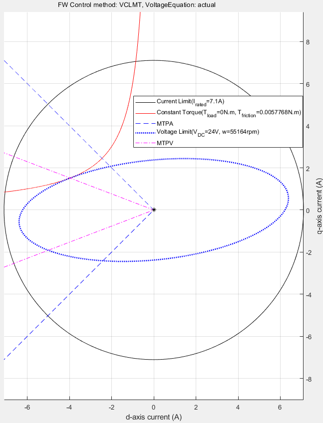
Figure 13: Constraint curves of a SynRM drawn at maximum operable speed, at 0 N.m. external load torque.

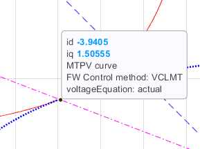
Figure 14: Zoomed-in portion from figure 13 to show the tangential intersection of two curves - voltage limit ellipse and constant torque curve.

Figure 15: Drive characteristics of the motor marked with a point at the maximum operable speed.

Finding Corner Speed of Motor

The rated speed of a motor is the speed at which the motor can be loaded with the rated torque, while operating at the rated voltage. This speed is also known as the corner speed because at this speed, speed-torque characteristics of a PMSM has a change of shape. For example, in figure 18, the highlighted point marks the corner speed of the motor. This speed is also known as the base speed. You can either use the analytical equations or the constraint curves to find the corner speed.

From the constraint curves, you can determine the corner speed of a machine, which is a point where the voltage limit curve crosses the intersection of the MTPA curve and the current limit circle. When the speed increases beyond the corner speed, the voltage limit curve does not enclose the intersection of the MTPA curve and the current limit circle.

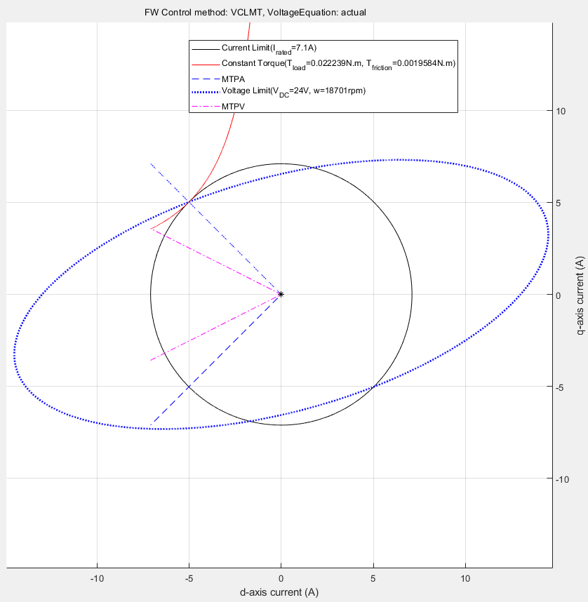
Figure 16: Constraint curves of a SynRM drawn at base speed (corner speed) and at rated torque.

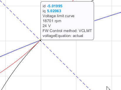
Figure 17: Zoomed in portion of figure 16 to show the intersection of MTPA curve, current limit circle, and voltage limit curve.

Figure 18: The speed-torque characteristics of a SynRM marked at corner speed and at rated torque.

Identifying Possible (MTPA-Field Weakening-MTPV) Control Currents

The preceding section showed that you can derive optimal (id, iq) values for different speeds and torques.

In a typical motor control application, you need a reference current value for the operating speed and reference torque. You can use the preceding methods to derive such reference currents, which result in optimal operations.

LUT based SynRM Control Reference

The block LUT based SynRM Control Reference computes the id and iq lookup tables using the given motor parameters (either linear lumped parameters or nonlinear parameter maps) or uses the user-provided id, iq lookup table values.

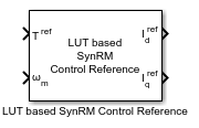
Figure 19: LUT based SynRM Control Reference block available in Motor Control Blockset library.

Figure 20: The mask view for the block with options showing the input possibilities for the motor parameters.

The LUT based SynRM Control reference block accepts multiple types of inputs that can utilize the externally generated id-iq LUTs or calculate the LUTs based on the provided motor parameters (linear or nonlinear). When you select the motor parameters (either linear or non-linear) as the parameter input method, the LUT based SynRM Control Reference block computes the LUTs on the host before the simulation begins or before the code-generation step.

mcbGenerateTables

You can use the function mcbGenerateTables available in Motor Control Blockset to create the id and iq LUTs on the host for custom grid sizes and grid point densities. The LUT based SynRM Control Reference block uses this function to compute the id and iq LUTs using the given motor parameters.

When the id and iq LUTs are generated, you can plot them in the d-q current space for multiple speed and torque values. When the point grid overlaps with the constraint curves of the motor, you can obtain figure 21. In the figure, the dots at the intersection of the curves are only for representation purposes. The output figure window of the function has segments of the voltage limit curve and constant torque curves that are drawn within the current limit circle.

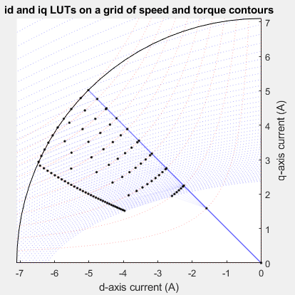
Figure 21: Grid of id, iq look-up tables for different speeds and load torques. This figure uses an axis notation that is identical to that of a PMSM.

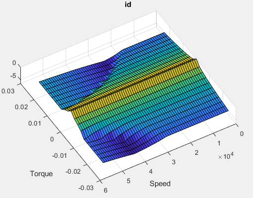
Figure 22: id LUT.

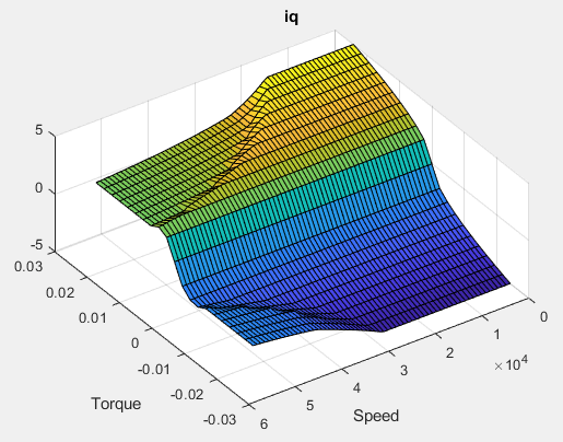
Figure 23: iq LUT.

For axis notation diferent from that of PMSM, you can obtain the following id and iq LUTs. Note that both id and iq remain positive.

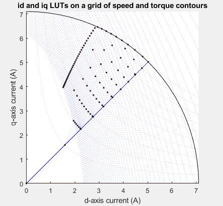
Figure 24: Grid of id-iq look-up tables for different speeds and load torques. This figure uses an axis notation that is different than that of a PMSM.