Solve Single PDE

This example shows how to formulate, compute, and plot the solution to a single PDE.

Consider the partial differential equation

$π^{2} \frac{\partial u}{\partial t} = \frac{\partial^{2} u}{\partial x^{2}} .$

The equation is defined on the interval $0 \leq x \leq 1$ for times $t \geq 0$ . At $t = 0$ , the solution satisfies the initial condition

$u (x, 0) = \sin (π x) .$

Also, at $x = 0$ and $x = 1$ , the solution satisfies the boundary conditions

$u (0, t) = 0,$

$π e^{- t} + \frac{\partial u}{\partial x} (1, t) = 0 .$

To solve this equation in MATLAB®, you need to code the equation, the initial conditions, and the boundary conditions, then select a suitable solution mesh before calling the solver pdepe. You either can include the required functions as local functions at the end of a file (as done here), or save them as separate, named files in a directory on the MATLAB path.

Code Equation

Before you can code the equation, you need to rewrite it in a form that the pdepe solver expects. The standard form that pdepe expects is

$c (x, t, u, \frac{\partial u}{\partial x}) \frac{\partial u}{\partial t} = x^{- m} \frac{\partial}{\partial x} (x^{m} f (x, t, u, \frac{\partial u}{\partial x})) + s (x, t, u, \frac{\partial u}{\partial x})$ .

Written in this form, the PDE becomes

$π^{2} \frac{\partial u}{\partial t} = x^{0} \frac{\partial}{\partial x} (x^{0} \frac{\partial u}{\partial x}) + 0$ .

With the equation in the proper form you can read off the relevant terms:

$m = 0$

$c (x, t, u, \frac{\partial u}{\partial x}) = π^{2}$

$f (x, t, u, \frac{\partial u}{\partial x}) = \frac{\partial u}{\partial x}$

$s (x, t, u, \frac{\partial u}{\partial x}) = 0$

Now you can create a function to code the equation. The function should have the signature [c,f,s] = pdex1pde(x,t,u,dudx):

x is the independent spatial variable.
t is the independent time variable.
u is the dependent variable being differentiated with respect to x and t.
dudx is the partial spatial derivative $\partial u / \partial x$ .
The outputs c, f, and s correspond to coefficients in the standard PDE equation form expected by pdepe. These coefficients are coded in terms of the input variables x, t, u, and dudx.

As a result, the equation in this example can be represented by the function:

function [c,f,s] = pdex1pde(x,t,u,dudx)
c = pi^2;
f = dudx;
s = 0;
end

(Note: All functions are included as local functions at the end of the example.)

Code Initial Condition

Next, write a function that returns the initial condition. The initial condition is applied at the first time value tspan(1). The function should have the signature u0 = pdex1ic(x).

The corresponding function is

function u0 = pdex1ic(x)
u0 = sin(pi*x);
end

Code Boundary Conditions

Now, write a function that evaluates the boundary conditions. For problems posed on the interval $a \leq x \leq b$ , the boundary conditions apply for all $t$ and either $x = a$ or $x = b$ . The standard form for the boundary conditions expected by the solver is

$p (x, t, u) + q (x, t) f (x, t, u, \frac{\partial u}{\partial x}) = 0 .$

Rewrite the boundary conditions in this standard form and read off the coefficient values.

For $x = 0$ , the equation is

$u (0, t) = 0 \to u + 0 \cdot \frac{\partial u}{\partial x} = 0 .$

The coefficients are:

$p (0, t, u) = u$
$q (0, t) = 0$

For $x = 1$ , the equation is

$π e^{- t} + \frac{\partial u}{\partial x} (1, t) = 0 \to π e^{- t} + 1 \cdot \frac{\partial u}{\partial x} (1, t) = 0 .$

The coefficients are:

$p (1, t, u) = π e^{- t}$
$q (1, t) = 1$

Since the boundary condition function is expressed in terms of $f (x, t, u, \frac{\partial u}{\partial x})$ , and this term is already defined in the main PDE function, you do not need to specify this piece of the equation in the boundary condition function. You need only specify the values of $p (x, t, u)$ and $q (x, t)$ at each boundary.

The boundary function should use the function signature [pl,ql,pr,qr] = pdex1bc(xl,ul,xr,ur,t):

The inputs xl and ul correspond to $u$ and $x$ for the left boundary.
The inputs xr and ur correspond to $u$ and $x$ for the right boundary.
t is the independent time variable.
The outputs pl and ql correspond to $p (x, t, u)$ and $q (x, t)$ for the left boundary ( $x = 0$ for this problem).
The outputs pr and qr correspond to $p (x, t, u)$ and $q (x, t)$ for the right boundary ( $x = 1$ for this problem).

The boundary conditions in this example are represented by the function:

function [pl,ql,pr,qr] = pdex1bc(xl,ul,xr,ur,t)
pl = ul;
ql = 0;
pr = pi * exp(-t);
qr = 1;
end

Select Solution Mesh

Before solving the equation you need to specify the mesh points $(t, x)$ at which you want pdepe to evaluate the solution. Specify the points as vectors t and x. The vectors t and x play different roles in the solver. In particular, the cost and accuracy of the solution depend strongly on the length of the vector x. However, the computation is much less sensitive to the values in the vector t.

For this problem, use a mesh with 20 equally spaced points in the spatial interval [0,1] and five values of t from the time interval [0,2].

x = linspace(0,1,20);
t = linspace(0,2,5);

Solve Equation

Finally, solve the equation using the symmetry m, the PDE equation, the initial conditions, the boundary conditions, and the meshes for x and t.

m = 0;
sol = pdepe(m,@pdex1pde,@pdex1ic,@pdex1bc,x,t);

pdepe returns the solution in a 3-D array sol, where sol(i,j,k) approximates the kth component of the solution $u_{k}$ evaluated at t(i) and x(j). The size of sol is length(t)-by-length(x)-by-length(u0), since u0 specifies an initial condition for each solution component. For this problem, u has only one component, so sol is a 5-by-20 matrix, but in general you can extract the kth solution component with the command u = sol(:,:,k).

Extract the first solution component from sol.

u = sol(:,:,1);

Plot Solution

Create a surface plot of the solution.

surf(x,t,u)
title('Numerical solution computed with 20 mesh points')
xlabel('Distance x')
ylabel('Time t')

Figure contains an axes object. The axes object with title Numerical solution computed with 20 mesh points, xlabel Distance x, ylabel Time t contains an object of type surface.

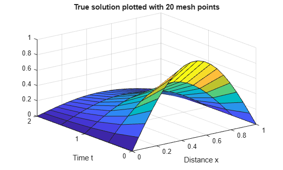
The initial condition and boundary conditions of this problem were chosen so that there would be an analytical solution, given by

$u (x, t) = e^{- t} \sin (π x) .$

Plot the analytical solution with the same mesh points.

surf(x,t,exp(-t)'*sin(pi*x))
title('True solution plotted with 20 mesh points')
xlabel('Distance x')
ylabel('Time t')

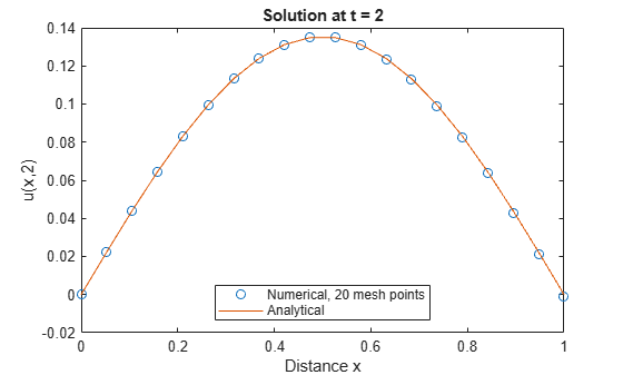
Figure contains an axes object. The axes object with title True solution plotted with 20 mesh points, xlabel Distance x, ylabel Time t contains an object of type surface.

Now, compare the numerical and analytical solutions at $t_{f}$ , the final value of $t$ . In this example $t_{f} = 2$ .

plot(x,u(end,:),'o',x,exp(-t(end))*sin(pi*x))
title('Solution at t = 2')
legend('Numerical, 20 mesh points','Analytical','Location','South')
xlabel('Distance x')
ylabel('u(x,2)')

Figure contains an axes object. The axes object with title Solution at t = 2, xlabel Distance x, ylabel u(x,2) contains 2 objects of type line. One or more of the lines displays its values using only markers These objects represent Numerical, 20 mesh points, Analytical.

Local Functions

Listed here are the local helper functions that the PDE solver pdepe calls to calculate the solution. Alternatively, you can save these functions as their own files in a directory on the MATLAB path.

function [c,f,s] = pdex1pde(x,t,u,dudx) % Equation to solve
c = pi^2;
f = dudx;
s = 0;
end
%----------------------------------------------
function u0 = pdex1ic(x) % Initial conditions
u0 = sin(pi*x);
end
%----------------------------------------------
function [pl,ql,pr,qr] = pdex1bc(xl,ul,xr,ur,t) % Boundary conditions
pl = ul;
ql = 0;
pr = pi * exp(-t);
qr = 1;
end
%----------------------------------------------