Constrained Delaunay Triangulation

Constrain edges in a 2-D triangulation by using the delaunayTriangulation class. This means you can choose a pair of points in the triangulation and constrain an edge to join those points. You can picture this as “forcing” an edge between one or more pairs of points. This example shows how edge constraints can affect the triangulation.

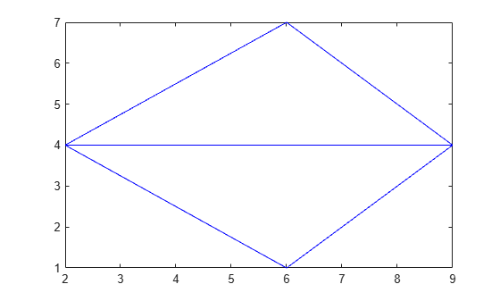
Triangulate a set of points with an edge constraint specified between vertex V1 and V3.

Define the point set.

P = [2 4;
     6 1;
     9 4;
     6 7];

Define a constraint, C, between V1 and V3.

C = [1 3];
DT = delaunayTriangulation(P,C);

Plot the triangulation and add annotations.

triplot(DT)

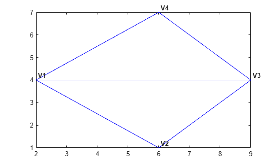
Label the vertices.

hold on
numvx = size(P,1);
vxlabels = arrayfun(@(n) {sprintf("V%d", n)},(1:numvx)');
Hpl = text(P(:,1)+0.2, P(:,2)+0.2, vxlabels, FontWeight="bold", ...
    HorizontalAlignment="center", BackgroundColor="none");
hold off

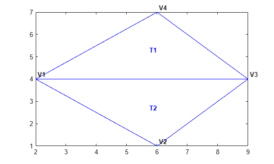
Use the incenters to find the positions for placing triangle labels on the plot.

hold on
IC = incenter(DT);
numtri = size(DT,1);
trilabels = arrayfun(@(P) {sprintf('T%d', P)},(1:numtri)');
Htl = text(IC(:,1),IC(:,2),trilabels,FontWeight="bold", ...
    HorizontalAlignment="center",Color="blue");
hold off

Plot the circumcircle associated with the triangle, T1.

hold on
[CC,r] = circumcenter(DT);
theta = 0:pi/50:2*pi;
xunit = r(1)*cos(theta) + CC(1,1);
yunit = r(1)*sin(theta) + CC(1,2);
plot(xunit,yunit,"g")
axis equal
hold off

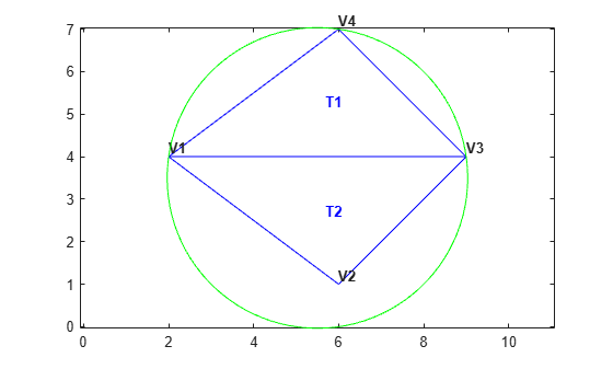
The constraint between vertices (V1, V3) was honored, however, the Delaunay criterion was invalidated. This also invalidates the nearest-neighbor relation that is inherent in a Delaunay triangulation. This means the nearestNeighbor search method provided by delaunayTriangulation cannot be supported if the triangulation has constraints.

In typical applications, the triangulation might be composed of many points, and a relatively small number of edges in the triangulation might be constrained. Such a triangulation is said to be locally non-Delaunay, because many triangles in the triangulation might respect the Delaunay criterion, but locally there might be some triangles that do not. In many applications, local relaxation of the empty circumcircle property is not a concern.

Constrained triangulations are generally used to triangulate a nonconvex polygon. The constraints give us a correspondence between the polygon edges and the triangulation edges. This relationship enables you to extract a triangulation that represents the region. The following example shows how to use a constrained delaunayTriangulation to triangulate a nonconvex polygon.

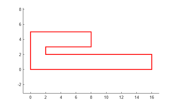
Define and plot a polygon.

figure()
axis([-1 17 -1 6]);
axis equal
P = [0  0;
     16 0;
     16 2;
     2  2;
     2  3;
     8  3;
     8  5;
     0  5];
patch(P(:,1),P(:,2),"r",LineWidth=2,FaceColor="none",EdgeColor="r");

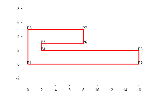
Label the points.

hold on
numvx = size(P,1);
vxlabels = arrayfun(@(n) {sprintf("P%d", n)},(1:numvx)');
Hpl = text(P(:,1)+0.2, P(:,2)+0.2, vxlabels,FontWeight="bold", ...
    HorizontalAlignment="center",BackgroundColor="none");
hold off

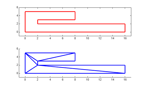
Create and plot the triangulation together with the polygon boundary.

figure()
subplot(2,1,1);
axis([-1 17 -1 6]);
axis equal

P = [0  0;
     16 0;
     16 2;
     2  2;
     2  3;
     8  3;
     8  5;
     0  5];
DT = delaunayTriangulation(P);
triplot(DT)
hold on
patch(P(:,1),P(:,2),"r",LineWidth=2,FaceColor="none",EdgeColor="r");
hold off

Plot the standalone triangulation in a subplot.

subplot(2,1,2);
axis([-1 17 -1 6]);
axis equal
triplot(DT)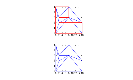

This triangulation cannot be used to represent the domain of the polygon because some triangles cut across the boundary. You need to impose a constraint on the edges that are cut by triangulation edges. Since all edges have to be respected, you need to constrain all edges. The steps below show how to constrain all the edges.

Enter the constrained edge definition. Observe from the annotated figure where you need constraints (between (V1, V2), (V2, V3), and so on).

C = [1 2;
     2 3;
     3 4;
     4 5;
     5 6;
     6 7;
     7 8;
     8 1];

In general, if you have N points in a sequence that define a polygonal boundary, the constraints can be expressed as C = [(1:(N-1))' (2:N)'; N 1];.

Specify the constraints when you create the delaunayTriangulation.

DT = delaunayTriangulation(P,C);

Alternatively, you can impose constraints on an existing triangulation by setting the Constraints property: DT.Constraints = C;.

Plot the triangulation and polygon.

figure(Color="white")
subplot(2,1,1);
axis([-1 17 -1 6]);
axis equal
triplot(DT)
hold on
patch(P(:,1),P(:,2),"r",LineWidth=2,FaceColor="none",EdgeColor="r"); 
hold off

Plot the standalone triangulation in a subplot.

subplot(2,1,2);
axis([-1 17 -1 6]);
axis equal
triplot(DT)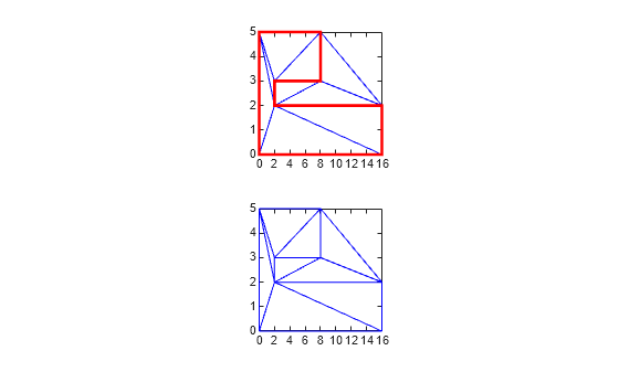

The plot shows that the edges of the triangulation respect the boundary of the polygon. However, the triangulation fills the concavities. What is needed is a triangulation that represents the polygonal domain. You can extract the triangles within the polygon using the delaunayTriangulation method, isInterior. This method returns a logical array whose true and false values that indicate whether the triangles are inside a bounded geometric domain. The analysis is based on the Jordan Curve theorem, and the boundaries are defined by the edge constraints. The ith triangle in the triangulation is considered to be inside the domain if the ith logical flag is true, otherwise it is outside.

Now use the isInterior method to compute and plot the set of domain triangles.

Plot the constrained edges in red.

figure(Color="white")
subplot(2,1,1);
plot(P(C'),P(C'+size(P,1)),"r",LineWidth=2);
axis([-1 17 -1 6]);

Compute the in/out status.

IO = isInterior(DT);
subplot(2,1,2);
hold on
axis([-1 17 -1 6]);

Use triplot to plot the triangles that are inside. Uses logical indexing and dt(i,j) shorthand format to access the triangulation.

triplot(DT(IO, :),DT.Points(:,1),DT.Points(:,2),LineWidth=2)
hold off