Sparse Matrix Reordering
This example shows how reordering the rows and columns of a sparse matrix can influence the speed and storage requirements of a matrix operation.
Visualizing a Sparse Matrix
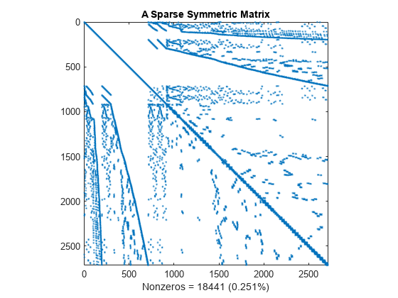
A spy plot shows the nonzero elements in a matrix.
This spy plot shows a sparse symmetric positive definite matrix derived from a portion of the barbell matrix. This matrix describes connections in a graph that resembles a barbell.
load barbellgraph.mat
S = A + speye(size(A));
pct = 100 / numel(A);
spy(S)
title('A Sparse Symmetric Matrix')
nz = nnz(S);
xlabel(sprintf('Nonzeros = %d (%.3f%%)',nz,nz*pct));
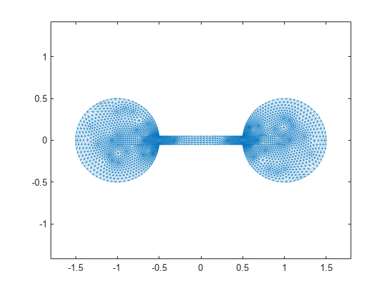
Here is a plot of the barbell graph.
G = graph(S,'omitselfloops');
p = plot(G,'XData',xy(:,1),'YData',xy(:,2),'Marker','.');
axis equal
Computing the Cholesky Factor
Compute the Cholesky factor L, where S = L*L'. Notice that L contains many more nonzero elements than the unfactored S, because the computation of the Cholesky factorization creates fill-in nonzeros. These fill-in values slow down the algorithm and increase storage cost.
L = chol(S,'lower');
spy(L)
title('Cholesky Decomposition of S')
nc(1) = nnz(L);
xlabel(sprintf('Nonzeros = %d (%.2f%%)',nc(1),nc(1)*pct));

Reordering to Speed Up Calculation
By reordering the rows and columns of a matrix, it is possible to reduce the amount of fill-in that factorization creates, thereby reducing the time and storage cost of subsequent calculations.
Several different reorderings supported by MATLAB® are:
colperm: Column countsymrcm: Reverse Cuthill-McKeeamd: Minimum degreedissect: Nested dissection
Test the effects of these sparse matrix reorderings on the barbell matrix.
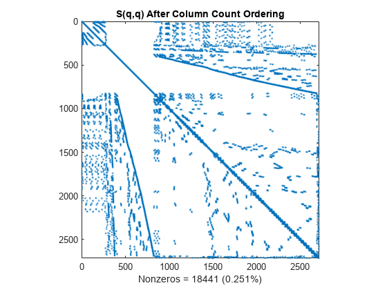
Column Count Reordering
The colperm command uses the column count reordering algorithm to move rows and columns with higher nonzero count towards the end of the matrix.
q = colperm(S);
spy(S(q,q))
title('S(q,q) After Column Count Ordering')
nz = nnz(S);
xlabel(sprintf('Nonzeros = %d (%.3f%%)',nz,nz*pct));
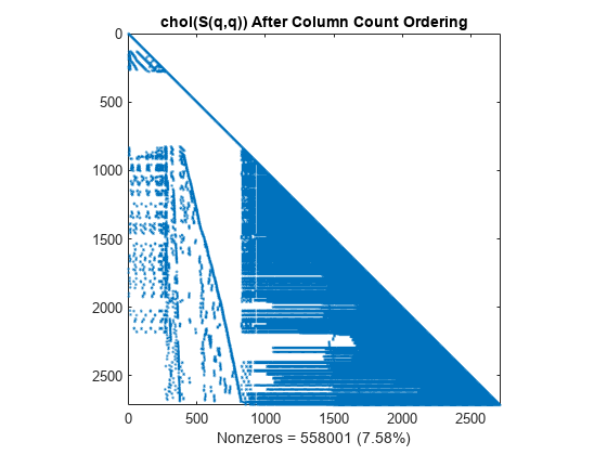
For this matrix, the column count ordering can barely reduce the time and storage for Cholesky factorization.
L = chol(S(q,q),'lower');
spy(L)
title('chol(S(q,q)) After Column Count Ordering')
nc(2) = nnz(L);
xlabel(sprintf('Nonzeros = %d (%.2f%%)',nc(2),nc(2)*pct));
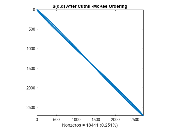
Reverse Cuthill-McKee Reordering
The symrcm command uses the reverse Cuthill-McKee reordering algorithm to move all nonzero elements closer to the diagonal, reducing the bandwidth of the original matrix.
d = symrcm(S);
spy(S(d,d))
title('S(d,d) After Cuthill-McKee Ordering')
nz = nnz(S);
xlabel(sprintf('Nonzeros = %d (%.3f%%)',nz,nz*pct));
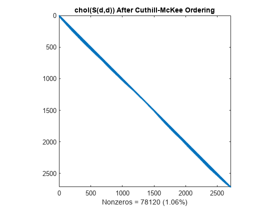
The fill-in produced by Cholesky factorization is confined to the band, so factorizing the reordered matrix takes less time and less storage.
L = chol(S(d,d),'lower');
spy(L)
title('chol(S(d,d)) After Cuthill-McKee Ordering')
nc(3) = nnz(L);
xlabel(sprintf('Nonzeros = %d (%.2f%%)', nc(3),nc(3)*pct));
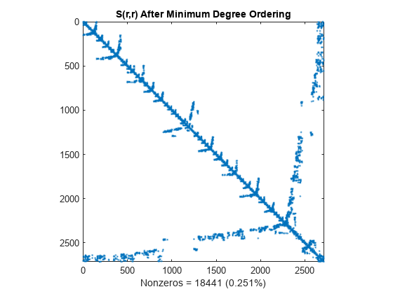
Minimum Degree Reordering
The amd command uses an approximate minimum degree algorithm (a powerful graph-theoretic technique) to produce large blocks of zeros in the matrix.
r = amd(S);
spy(S(r,r))
title('S(r,r) After Minimum Degree Ordering')
nz = nnz(S);
xlabel(sprintf('Nonzeros = %d (%.3f%%)',nz,nz*pct));
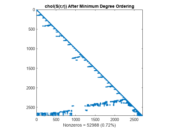
The Cholesky factorization preserves the blocks of zeros produced by the minimum degree algorithm. This structure can significantly reduce time and storage costs.
L = chol(S(r,r),'lower');
spy(L)
title('chol(S(r,r)) After Minimum Degree Ordering')
nc(4) = nnz(L);
xlabel(sprintf('Nonzeros = %d (%.2f%%)',nc(4),nc(4)*pct));
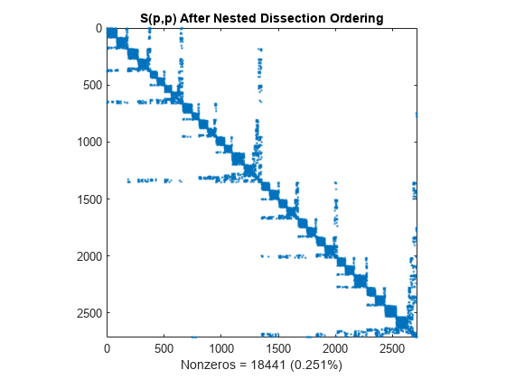
Nested Dissection Permutation
The dissect function uses graph-theoretic techniques to produce fill-reducing orderings. The algorithm treats the matrix as the adjacency matrix of a graph, coarsens the graph by collapsing vertices and edges, reorders the smaller graph, and then uses refinement steps to uncoarsen the small graph and produce a reordering of the original graph. The result is a powerful algorithm that frequently produces the least amount of fill-in compared to the other reordering algorithms.
p = dissect(S);
spy(S(p,p))
title('S(p,p) After Nested Dissection Ordering')
nz = nnz(S);
xlabel(sprintf('Nonzeros = %d (%.3f%%)',nz,nz*pct));
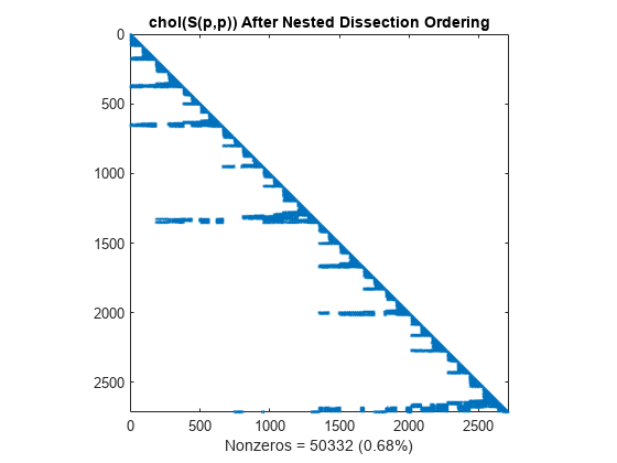
Similar to the minimum degree ordering, the Cholesky factorization of the nested dissection ordering mostly preserves the nonzero structure of S(d,d) below the main diagonal.
L = chol(S(p,p),'lower');
spy(L)
title('chol(S(p,p)) After Nested Dissection Ordering')
nc(5) = nnz(L);
xlabel(sprintf('Nonzeros = %d (%.2f%%)',nc(5),nc(5)*pct));
Summarizing Results
This bar chart summarizes the effects of reordering the matrix before performing the Cholesky factorization. While the Cholesky factorization of the original matrix had about 8% of its elements as nonzeros, using dissect or symamd reduces that density to less than 1%.
labels = {'Original','Column Count','Cuthill-McKee',...
    'Min Degree','Nested Dissection'};
bar(nc*pct)
title('Nonzeros After Cholesky Factorization')
ylabel('Percent');
ax = gca;
ax.XTickLabel = labels;
ax.XTickLabelRotation = -45;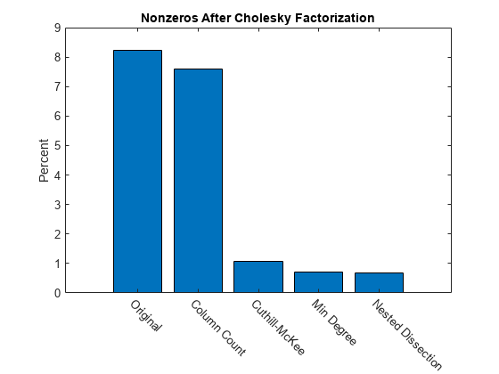
See Also
You can also select a web site from the following list:
Americas
- América Latina (Español)
- Canada (English)
- United States (English)
Europe
- Belgium (English)
- Denmark (English)
- Deutschland (Deutsch)
- España (Español)
- Finland (English)
- France (Français)
- Ireland (English)
- Italia (Italiano)
- Luxembourg (English)
- Netherlands (English)
- Norway (English)
- Österreich (Deutsch)
- Portugal (English)
- Sweden (English)
- Switzerland
- United Kingdom (English)