Analyze Big Data in MATLAB Using MapReduce
This example shows how to use the mapreduce function to process a large amount of file-based data. The MapReduce algorithm is a mainstay of many modern "big data" applications. This example operates on a single computer, but the code can scale up to use Hadoop®.
Throughout this example, the data set is a collection of records from the American Statistical Association for USA domestic airline flights between 1987 and 2008. If you have experimented with "big data" before, you may already be familiar with this data set. A small subset of this data set is included with MATLAB® to allow you to run this and other examples.
Introduction to Datastores
Creating a datastore allows you to access a collection of data in a block-based manner. A datastore can process arbitrarily large amounts of data, and the data can even be spread across multiple files. You can create a datastore for many file types, including a collection of tabular text files (demonstrated here), a SQL database (Database Toolbox™ required) or a Hadoop® Distributed File System (HDFS™).
Create a datastore for a collection of tabular text files and preview the contents.
ds = tabularTextDatastore('airlinesmall.csv');
dsPreview = preview(ds);
dsPreview(:,10:15)ans=8×6 table
FlightNum TailNum ActualElapsedTime CRSElapsedTime AirTime ArrDelay
_________ _______ _________________ ______________ _______ ________
1503 {'NA'} 53 57 {'NA'} 8
1550 {'NA'} 63 56 {'NA'} 8
1589 {'NA'} 83 82 {'NA'} 21
1655 {'NA'} 59 58 {'NA'} 13
1702 {'NA'} 77 72 {'NA'} 4
1729 {'NA'} 61 65 {'NA'} 59
1763 {'NA'} 84 79 {'NA'} 3
1800 {'NA'} 155 143 {'NA'} 11
The datastore automatically parses the input data and makes a best guess as to the type of data in each column. In this case, use the 'TreatAsMissing' name-value pair argument to replace the missing values correctly. For numeric variables (such as 'AirTime'), tabularTextDatastore replaces every instance of 'NA' with a NaN value, which is the IEEE arithmetic representation for Not-a-Number.
ds = tabularTextDatastore('airlinesmall.csv', 'TreatAsMissing', 'NA');
ds.SelectedFormats{strcmp(ds.SelectedVariableNames, 'TailNum')} = '%s';
ds.SelectedFormats{strcmp(ds.SelectedVariableNames, 'CancellationCode')} = '%s';
dsPreview = preview(ds);
dsPreview(:,{'AirTime','TaxiIn','TailNum','CancellationCode'})
ans=8×4 table
    AirTime    TaxiIn    TailNum    CancellationCode
    _______    ______    _______    ________________

      NaN       NaN      {'NA'}          {'NA'}
      NaN       NaN      {'NA'}          {'NA'}
      NaN       NaN      {'NA'}          {'NA'}
      NaN       NaN      {'NA'}          {'NA'}
      NaN       NaN      {'NA'}          {'NA'}
      NaN       NaN      {'NA'}          {'NA'}
      NaN       NaN      {'NA'}          {'NA'}
      NaN       NaN      {'NA'}          {'NA'}
Scan for rows of interest
Datastore objects contain an internal pointer to keep track of which block of data the read function returns next. Use the hasdata and read functions to step through the entire data set, and filter the data set to only the rows of interest. In this case, the rows of interest are flights on United Airlines ("UA") departing from Boston ("BOS").
subset = [];

while hasdata(ds)
    t = read(ds);
    t = t(strcmp(t.UniqueCarrier, 'UA') & strcmp(t.Origin, 'BOS'), :);
    subset = vertcat(subset, t);
end

subset(1:10,[9,10,15:17])
ans=10×5 table
    UniqueCarrier    FlightNum    ArrDelay    DepDelay    Origin
    _____________    _________    ________    ________    _______

       {'UA'}           121          -9           0       {'BOS'}
       {'UA'}          1021          -9          -1       {'BOS'}
       {'UA'}           519          15           8       {'BOS'}
       {'UA'}           354           9           8       {'BOS'}
       {'UA'}           701         -17           0       {'BOS'}
       {'UA'}           673          -9          -1       {'BOS'}
       {'UA'}            91          -3           2       {'BOS'}
       {'UA'}           335          18           4       {'BOS'}
       {'UA'}          1429           1          -2       {'BOS'}
       {'UA'}            53          52          13       {'BOS'}
Introduction to mapreduce
MapReduce is an algorithmic technique to "divide and conquer" big data problems. In MATLAB, mapreduce requires three input arguments:
A datastore to read data from
A "mapper" function that is given a subset of the data to operate on. The output of the map function is a partial calculation.
mapreducecalls the mapper function one time for each block in the datastore, with each call operating independently.A "reducer" function that is given the aggregate outputs from the mapper function. The reducer function finishes the computation begun by the mapper function, and outputs the final answer.
This is an over-simplification to some extent, since the output of a call to the mapper function can be shuffled and combined in interesting ways before being passed to the reducer function. This will be examined later in this example.
Use mapreduce to perform a computation
A simple use of mapreduce is to find the longest flight time in the entire airline data set. To do this:
The "mapper" function computes the maximum of each block from the datastore.
The "reducer" function then computes the maximum value among all of the maxima computed by the calls to the mapper function.
First, reset the datastore and filter the variables to the one column of interest.
reset(ds);
ds.SelectedVariableNames = {'ActualElapsedTime'};
Write the mapper function, maxTimeMapper.m. It takes three input arguments:
The input data, which is a table obtained by applying the
readfunction to the datastore.A collection of configuration and contextual information,
info. This can be ignored in most cases, as it is here.An intermediate data storage object, which records the results of the calculations from the mapper function. Use the
addfunction to add Key/Value pairs to this intermediate output. In this example, the name of the key ('MaxElapsedTime') is arbitrary.
Save the following mapper function (maxTimeMapper.m) in your current folder.
function maxTimeMapper(data, ~, intermKVStore)
  maxElapsedTime = max(data{:,:});
  add(intermKVStore, "MaxElapsedTime", maxElapsedTime)
end
Next, write the reducer function. It also takes three input arguments:
A set of input "keys". Keys will be discussed further below, but they can be ignored in some simple problems, as they are here.
An intermediate data input object that
mapreducepasses to the reducer function. This data is in the form of Key/Value pairs, and you use thehasnextandgetnextfunctions to iterate through the values for each key.A final output data storage object. Use the
addandaddmultifunctions to directly add Key/Value pairs to the output.
Save the following reducer function (maxTimeReducer.m) in your current folder.
function maxTimeReducer(~, intermValsIter, outKVStore)
  maxElapsedTime = -Inf;
  while(hasnext(intermValsIter))
    maxElapsedTime = max(maxElapsedTime, getnext(intermValsIter));
  end
  add(outKVStore, "MaxElapsedTime", maxElapsedTime);
end
Once the mapper and reducer functions are written and saved in your current folder, you can call mapreduce using the datastore, mapper function, and reducer function. If you have Parallel Computing Toolbox (PCT), MATLAB will automatically start a pool and parallelize execution. Use the readall function to display the results of the MapReduce algorithm.
result = mapreduce(ds, @maxTimeMapper, @maxTimeReducer);
********************************
*      MAPREDUCE PROGRESS      *
********************************
Map   0% Reduce   0%
Map  16% Reduce   0%
Map  32% Reduce   0%
Map  48% Reduce   0%
Map  65% Reduce   0%
Map  81% Reduce   0%
Map  97% Reduce   0%
Map 100% Reduce   0%
Map 100% Reduce 100%
readall(result)
ans=1×2 table
           Key             Value
    __________________    ________

    {'MaxElaspedTime'}    {[1650]}
Use of keys in mapreduce
The use of keys is an important and powerful feature of mapreduce. Each call to the mapper function adds intermediate results to one or more named "buckets", called keys. The number of calls to the mapper function by mapreduce corresponds to the number of blocks in the datastore.
If the mapper function adds values to multiple keys, this leads to multiple calls to the reducer function, with each call working on only one key's intermediate values. The mapreduce function automatically manages this data movement between the map and reduce phases of the algorithm.
This flexibility is useful in many contexts. The example below uses keys in a relatively obvious way for illustrative purposes.
Calculating group-wise metrics with mapreduce
The behavior of the mapper function in this application is more complex. For every flight carrier found in the input data, use the add function to add a vector of values. This vector is a count of the number of flights for that carrier on each day in the 21+ years of data. The carrier code is the key for this vector of values. This ensures that all of the data for each carrier will be grouped together when mapreduce passes it to the reducer function.
Save the following mapper function (countFlightsMapper.m) in your current folder.
function countFlightsMapper(data, ~, intermKVStore)
  dayNumber = days((datetime(data.Year, data.Month, data.DayofMonth) - datetime(1987,10,1)))+1;
  daysSinceEpoch = days(datetime(2008,12,31) - datetime(1987,10,1))+1;
  [airlineName, ~, airlineIndex] = unique(data.UniqueCarrier, 'stable');

  for i = 1:numel(airlineName)
    dayTotals = accumarray(dayNumber(airlineIndex==i), 1, [daysSinceEpoch, 1]);
    add(intermKVStore, airlineName{i}, dayTotals);
  end
end
The reducer function is less complex. It simply iterates over the intermediate values and adds the vectors together. At completion, it outputs the values in this aggregate vector. Note that the reducer function does not need to sort or examine the intermediateKeysIn values; each call to the reducer function by mapreduce only passes the values for one airline carrier.
Save the following reducer function (countFlightsReducer.m) in your current folder.
function countFlightsReducer(intermKeysIn, intermValsIter, outKVStore)
  daysSinceEpoch = days(datetime(2008,12,31) - datetime(1987,10,1))+1;
  dayArray = zeros(daysSinceEpoch, 1);

  while hasnext(intermValsIter)
    dayArray = dayArray + getnext(intermValsIter);
  end
  add(outKVStore, intermKeysIn, dayArray);
end
Reset the datastore and select the variables of interest. Once the mapper and reducer functions are written and saved in your current folder, you can call mapreduce using the datastore, mapper function, and reducer function.
reset(ds);
ds.SelectedVariableNames = {'Year', 'Month', 'DayofMonth', 'UniqueCarrier'};
result = mapreduce(ds, @countFlightsMapper, @countFlightsReducer);
******************************** * MAPREDUCE PROGRESS * ******************************** Map 0% Reduce 0% Map 16% Reduce 0% Map 32% Reduce 0% Map 48% Reduce 0% Map 65% Reduce 0% Map 81% Reduce 0% Map 97% Reduce 0% Map 100% Reduce 0% Map 100% Reduce 10% Map 100% Reduce 21% Map 100% Reduce 31% Map 100% Reduce 41% Map 100% Reduce 52% Map 100% Reduce 62% Map 100% Reduce 72% Map 100% Reduce 83% Map 100% Reduce 93% Map 100% Reduce 100%
result = readall(result);
In case this example was run with only the sample data set, load the results of the mapreduce algorithm run on the entire data set.
load airlineResultsVisualizing the results
Using only the top 7 carriers, smooth the data to remove the effects of weekend travel. This would otherwise clutter the visualization.
lines = result.Value;
lines = horzcat(lines{:});
[~,sortOrder] = sort(sum(lines), 'descend');
lines = lines(:,sortOrder(1:7));
result = result(sortOrder(1:7),:);

lines(lines==0) = nan;
lines = smoothdata(lines,'gaussian');
Plot the data.
figure('Position',[1 1 800 600]);
plot(datetime(1987,10,1):caldays(1):datetime(2008,12,31),lines,'LineWidth',2)
title ('Domestic airline flights per day per carrier')
xlabel('Date')
ylabel('Flights per day')
legend(result.Key, 'Location', 'Best')
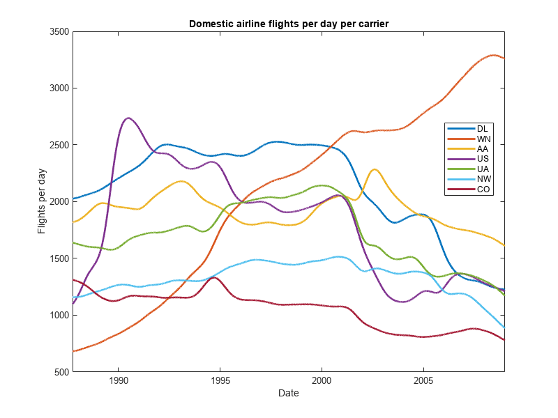
The plot shows the emergence of Southwest Airlines (WN) during this time period.
Learning more
This example only scratches the surface of what is possible with mapreduce. See the documentation for mapreduce for more information, including information on using it with Hadoop and MATLAB® Parallel Server™.
See Also
mapreduce | tabularTextDatastore
Related Topics
You can also select a web site from the following list:
Americas
- América Latina (Español)
- Canada (English)
- United States (English)
Europe
- Belgium (English)
- Denmark (English)
- Deutschland (Deutsch)
- España (Español)
- Finland (English)
- France (Français)
- Ireland (English)
- Italia (Italiano)
- Luxembourg (English)
- Netherlands (English)
- Norway (English)
- Österreich (Deutsch)
- Portugal (English)
- Sweden (English)
- Switzerland
- United Kingdom (English)