Color Analysis with Bivariate Histogram
This example shows how to adjust the color scale of a bivariate histogram plot to reveal additional details about the bins.
Load the image peppers.png, which is a color photo of several types of peppers and other vegetables. The unsigned 8-bit integer array rgb contains the image data.
rgb = imread('peppers.png');
imshow(rgb)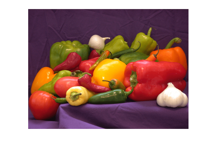
Plot a bivariate histogram of the red and green RGB values for each pixel to visualize the color distribution.
r = rgb(:,:,1);
g = rgb(:,:,2);
b = rgb(:,:,3);
histogram2(r,g,'DisplayStyle','tile','ShowEmptyBins','on', ...
    'XBinLimits',[0 255],'YBinLimits',[0 255]);
axis equal
colorbar
xlabel('Red Values')
ylabel('Green Values')
title('Green vs. Red Pixel Components')
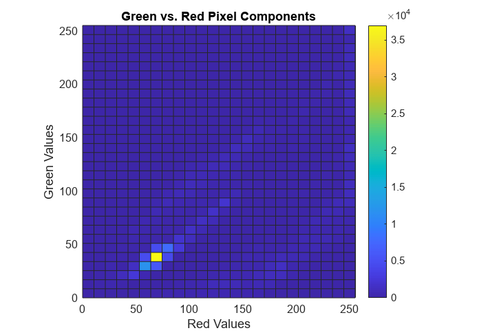
The histogram is heavily weighted towards the bottom of the color scale because there are a few bins with very large counts. This results in most of the bins displaying as the first color in the colormap, blue. Without additional detail it is hard to draw any conclusions about which color is more dominant.
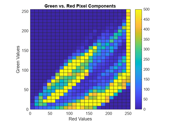
To view more detail, rescale the histogram color scale by setting the CLim property of the axes to have a range between 0 and 500. The result is that the histogram bins whose count is 500 or greater display as the last color in the colormap, yellow. Since most of the bin counts are within this smaller range, there is greater variation in the color of bins displayed.
ax = gca;
ax.CLim = [0 500];
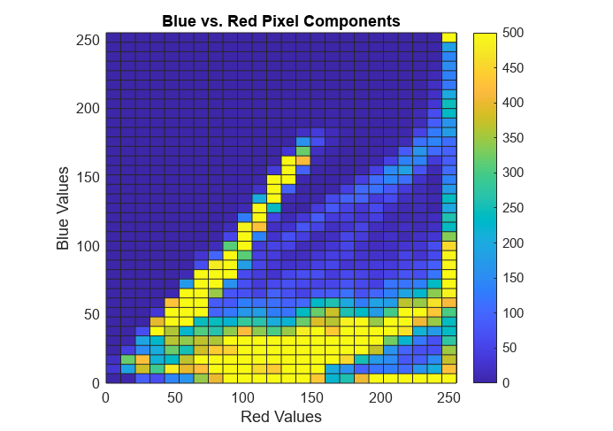
Use a similar method to compare the dominance of red vs. blue and green vs. blue.
histogram2(r,b,'DisplayStyle','tile','ShowEmptyBins','on',...
    'XBinLimits',[0 255],'YBinLimits',[0 255]);
axis equal
colorbar
xlabel('Red Values')
ylabel('Blue Values')
title('Blue vs. Red Pixel Components')
ax = gca;
ax.CLim = [0 500];
histogram2(g,b,'DisplayStyle','tile','ShowEmptyBins','on',...
    'XBinLimits',[0 255],'YBinLimits',[0 255]);
axis equal
colorbar
xlabel('Green Values')
ylabel('Blue Values')
title('Green vs. Blue Pixel Components')
ax = gca;
ax.CLim = [0 500];
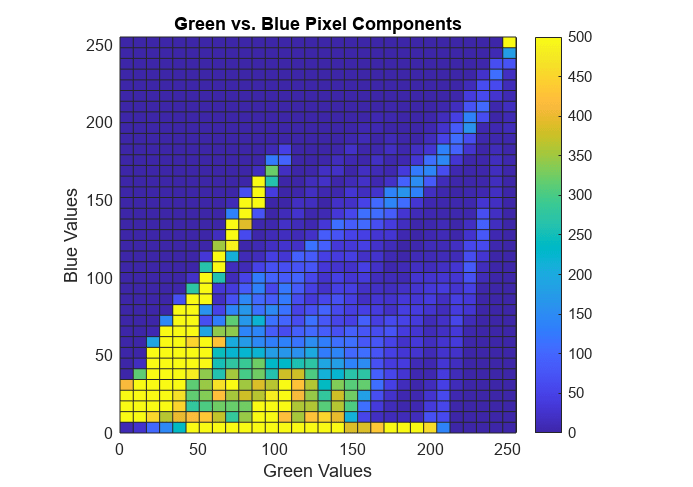
In each case, blue is the least dominant color signal. Looking at all three histograms, red appears to be the dominant color.
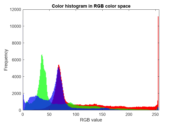
Confirm the results by creating a color histogram in the RGB color space. All three color components have spikes for smaller RGB values. However, the values above 100 occur more frequently in the red component than any other.
histogram(r,'BinMethod','integers','FaceColor','r','EdgeAlpha',0,'FaceAlpha',1)
hold on
histogram(g,'BinMethod','integers','FaceColor','g','EdgeAlpha',0,'FaceAlpha',0.7)
histogram(b,'BinMethod','integers','FaceColor','b','EdgeAlpha',0,'FaceAlpha',0.7)
xlabel('RGB value')
ylabel('Frequency')
title('Color histogram in RGB color space')
xlim([0 257])