Texture Segmentation Using Gabor Filters
This example shows how to use texture segmentation to identify regions based on their texture. The goal is to segment the dog from the bathroom floor. The segmentation is visually obvious because of the difference in texture between the regular, periodic pattern of the bathroom floor, and the regular, smooth texture of the dog's fur.
Gabor filters are a reasonable model of simple cells in the mammalian vision system. Because of this, Gabor filters are thought to be a good model of how humans distinguish texture, and are therefore a useful model to use when designing algorithms to recognize texture.
Read Input Image
Read and display the input image. This example shrinks the image to make the example run more quickly.
A = imread("kobi.png");
A = imresize(A,0.25);
imshow(A)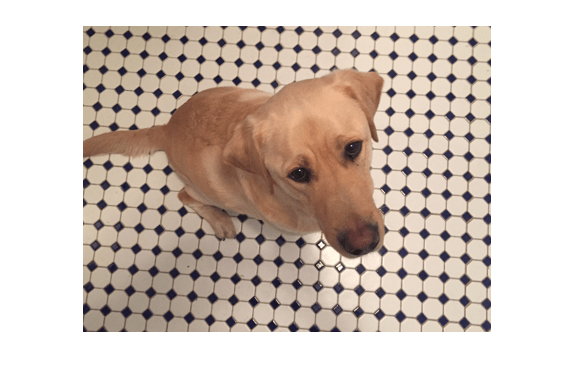
Design Array of Gabor Filters
Design an array of Gabor filters that are tuned to different frequencies and orientations [1]. The set of frequencies and orientations is designed to localize different, roughly orthogonal, subsets of frequency and orientation information in the input image. Sample orientations between 0 degrees and 135 degrees in steps of 45 degrees. Sample wavelength in increasing powers of two starting from 4/sqrt(2) up to the hypotenuse length of the input image.
[numRows,numCols,~] = size(A);

wavelengthMin = 4/sqrt(2);
wavelengthMax = hypot(numRows,numCols);
n = floor(log2(wavelengthMax/wavelengthMin));
wavelength = 2.^(0:(n-2)) * wavelengthMin;

deltaTheta = 45;
orientation = 0:deltaTheta:(180-deltaTheta);

g = gabor(wavelength,orientation);
Calculate Gabor Magnitude Response
Calculate the magnitude response of the Gabor filters from the source image by using the imgaborfilt function. The Gabor magnitude response is sometimes referred to as "Gabor Energy". Each Gabor magnitude response in gabormag(:,:,ind) is the output of the corresponding Gabor filter g(ind) as applied to the grayscale source image.
Agray = im2gray(A);
gabormag = imgaborfilt(Agray,g);
Create Feature Set
Post-process the Gabor magnitude responses for use in classification. This post processing includes Gaussian smoothing and adding additional spatial information to the feature set.
Each Gabor magnitude response contains some local variations, even within well-segmented regions of constant texture. These local variations will throw off the segmentation. Compensate for these variations by smoothing the Gabor magnitude information using Gaussian low-pass filters. Apply a different Gaussian filter to each Gabor magnitude response, and match the standard deviation of each Gaussian filter to the wavelength of the Gabor filter that produced the corresponding response. Control the amount of smoothing that is applied to the Gabor magnitude responses by using a smoothing term K.
K = 3;
for i = 1:length(g)
    sigma = 0.5*g(i).Wavelength;
    gabormag(:,:,i) = imgaussfilt(gabormag(:,:,i),K*sigma);
end
Supplement the Gabor feature set with a map of spatial location information in both X and Y. This additional information enables the classifier to prefer groupings that are close together spatially.
X = 1:numCols;
Y = 1:numRows;
[X,Y] = meshgrid(X,Y);
featureSet = cat(3,gabormag,X,Y);
In this example, there is a separate feature for each filter in the Gabor filter bank, plus two additional features from the spatial information that was added in the previous step. In total, there are 24 Gabor features and 2 spatial features for each pixel in the input image.
Visualize the Feature Set
Normalize the features to be zero mean, unit variance. To simplify the calculation, first reshape the feature set into a 2-D matrix with 26 columns. In this format, there is one column for each feature, and you can perform columnwise calculations of mean and standard deviation. After you have normalized the features, reshape the matrix to its original 3-D shape.
X = reshape(featureSet,numRows*numCols,[]);
Xnorm = (X-mean(X))./std(X);
featureSetNorm = reshape(Xnorm,numRows,numCols,[]);
Display the normalized features as a montage.
montage(featureSetNorm,[],Size=[5 6],Background="w")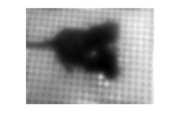
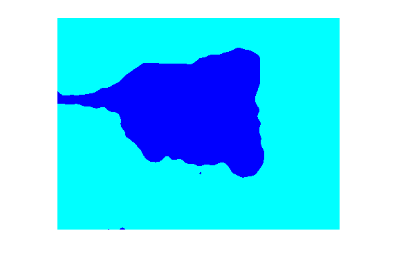
Classify Features
Segment the feature set into two clusters by using the imsegkmeans function. Normalize each feature independently by specifying the NormalizeInput name-value argument as true. To avoid local minima when minimizing the objective function, repeat the k-means clustering process five times.
featureSet = im2single(featureSet);
L = imsegkmeans(featureSet,2,NormalizeInput=true,NumAttempts=5);
Display the segmentation labels over the image using labeloverlay.
imshow(labeloverlay(A,L))
Examine the foreground and background images that result from the mask BW that is associated with the label matrix L.
Aseg1 = zeros(size(A),"like",A);
Aseg2 = zeros(size(A),"like",A);
BW = L == 2;
BW = repmat(BW,[1 1 3]);
Aseg1(BW) = A(BW);
Aseg2(~BW) = A(~BW);
montage({Aseg1,Aseg2});

References
[1]