Nonlinear ARX Model of SI Engine Torque Dynamics
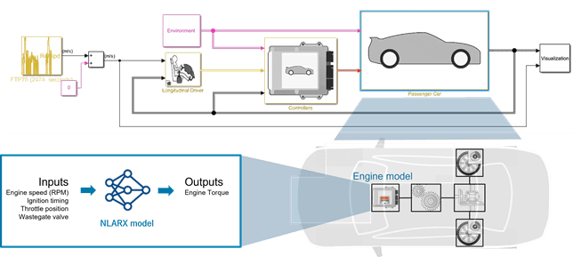
This example describes modeling the nonlinear torque dynamics of a spark-ignition (SI) engine as a nonlinear ARX model. The identified model can be used for hardware-in-the-loop (HIL) testing, powertrain control, diagnostic, and training algorithm design. For example, you can use the model for aftertreatment control and diagnostics algorithm development. For more information on nonlinear ARX models, see Nonlinear ARX Models.
You use measurements of the system inputs and outputs to identify the model. This data can come from measurements on a real engine or a high-fidelity model such as one created using the Powertrain Blockset™ SI Reference application.
Data Preparation
Load and display the engine data timetable.
load SIEngineData IOData
stackedplot(IOData)
title('SI Engine Signals')

The timetable contains over one hundred thousands observations of five variables measured at 10 Hz.
Throttle position (degrees)
Wastegate valve area (aperture percentage)
Engine speed (RPM)
Spark timing (degrees)
Engine torque (N m)
Split the data into estimation (first 60000 data points) and validation (remaining data points) portions.
eData = IOData(1:6e4,:);     % portion used for estimation
vData = IOData(6e4+1:end,:); % portion used for validation
Downsample the training data by a factor of 10. This helps speed up the model training process and also limits the focus of the fit to a lower frequency region.
% Downsample datasets 10 times
eDataD = idresamp(eData,[1 10]);
vDataD = idresamp(vData,[1 10]);
eDataD.Properties.TimeStep
ans = duration
1 sec
The model training objective is to generate a dynamic system that has the engine torque as output and the other four variables as inputs.
Nonlinear ARX Model Identification
About Nonlinear ARX Models
A nonlinear ARX model implements a two-stage transformation of the observed data to predict the future values. In the first step, it transforms the input/output signals into a finite-dimensional regressors, which are features based on time-delayed values of the signals. These regressors are mapped to the predicted output using a nonlinear but static function. You have many choices for the regressor formulas and the nonlinear functions.
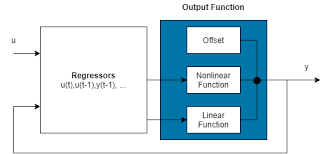
You can use linear, polynomial, or trigonometric transformations of the time-delayed variables. You can also use your physical insight to define your own custom regressors. The functions that map the regressors to the outputs usually employ a parallel connection combination of a linear function, a nonlinear function and an offset (bias) term. You can choose the nonlinear functions to be sigmoid or wavelet based networks, a Gaussian process (GP) function, support vector regression (SVM) functions, regression tree ensembles (bagging or boosting forms), or other basis function expansions expressed in terms of custom unit functions.
In this example, you identify nonlinear ARX models based on different nonlinear functions. Begin by designating the input and output signals from the list of variables in the eData timetable.
Inputs = ["ThrottlePosition","WastegateValve","EngineSpeed","SparkTiming"];
Output = "EngineTorque";
Sigmoid Network Model
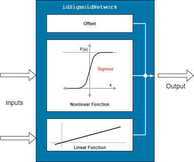
A sigmoid network model is a nonlinear ARX model that employs a parallel combination of a linear function, an offset term (bias), and a nonlinear function represented by a sum of dilated and translated sigmoid functions. The sigmoid network is represented by the idSigmoidNetwork object.
The parameters of the nonlinear ARX model are composed of parameters of the linear function, the nonlinear function and the offset. The modeling approach used in this example is incremental. You first estimate a linear, four-input, one-output model for the torque dynamics. Then, you extend the linear block by adding a single-hidden-layer sigmoid network to it in a parallel configuration to create a nonlinear ARX model.
Initial Linear Model
Create an object to specify options for estimating state-space models, and specify the option to minimize the simulation error (instead of the prediction error) during estimation.
ssOpt = ssestOptions(Focus="simulation");You can uncomment and run the following command to launch an interactive plot for selecting both the optimal order and the corresponding N4Horizon parameter value.
% linsys = ssest(eDataD, 1:10, ...
%   'Feedthrough',true(1,4), ...
%   'Ts',1, ...
%   'DisturbanceModel','none', ...
%   'InputName',Inputs, ...
%   'OutputName',Output, ...
%   ssOpt);
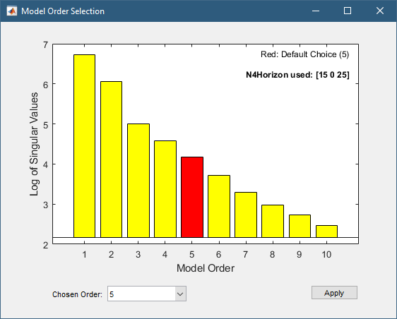
When you click Apply, an identified state-space model with your chosen order (here, 5) is created. Use the following commands to directly create this model without using the plot.
% Specify the horizon and the order
ssOpt.N4Horizon = [15 0 25];
Order = 5;

% Estimate the linear system
linsys = ssest(eDataD, Order, ...
'Feedthrough',true(1,4), ...
'Ts',1,...
'DisturbanceModel','none',...
'InputName',Inputs,...
'OutputName',Output,...
ssOpt)
linsys =
  Discrete-time identified state-space model:
    x(t+Ts) = A x(t) + B u(t) + K e(t)
       y(t) = C x(t) + D u(t) + e(t)

  A =
             x1        x2        x3        x4        x5
   x1     0.685   -0.2061    0.2727    0.1345    0.1283
   x2    0.3301  -0.01208    0.6969    0.2742    0.3221
   x3    0.0977    0.3312    0.4462   -0.5481   0.07495
   x4   -0.1477   -0.1594    0.9024   -0.2664    0.0361
   x5    0.0135     0.606   -0.4236   -0.2822    0.6817

  B =
       ThrottlePosi  WastegateVal   EngineSpeed   SparkTiming
   x1     0.0004832      -0.01389     0.0007426      0.001756
   x2      0.004744      -0.08037      0.004403      0.008711
   x3      0.002218      -0.04952      0.002774      0.002881
   x4      0.002496      -0.04896      0.002671      0.003919
   x5     -0.002972        0.0553     -0.003039     -0.005904

  C =
                     x1      x2      x3      x4      x5
   EngineTorque  -557.9   175.6  -85.25   10.78   49.91

  D =
                 ThrottlePosi  WastegateVal   EngineSpeed   SparkTiming
   EngineTorque        0.1519        0.1686      0.001073       0.05432

  K =
       EngineTorque
   x1             0
   x2             0
   x3             0
   x4             0
   x5             0

Sample time: 1 seconds

Parameterization:
   FREE form (all coefficients in A, B, C free).
   Feedthrough: yes
   Disturbance component: none
   Number of free coefficients: 54
   Use "idssdata", "getpvec", "getcov" for parameters and their uncertainties.

Status:
Estimated using SSEST on time domain data "eDataD".
Fit to estimation data: 46.45%
FPE: 173, MSE: 171.3

Model Properties
Compare the simulated response of linsys against the measured engine torque used for training.
clf
compare(eDataD, linsys)

The linear model is able to emulate the measured output, but with about a normalized root mean squared error (NRMSE) of 50%. However, as shown next, this linear model provides an excellent starting point for building a nonlinear ARX model.
Creating the Nonlinear Model
In the Sigmoid network based nonlinear ARX model, you have the option of disabling the linear function, the offset term, or both. You can also pick how many sigmoid units the nonlinear function employs. In this example, you retain the linear component and the offset term but change the number of sigmoid units to 11 (default is 10). The number of coefficients in the linear term and their initial values are set by using in the linear model linsys in the call to the model training command nlarx.
Create the nonlinear sigmoid-based function.
NumberOfUnits = 11; % determined by trial and error
NonlinearFcn = idSigmoidNetwork(NumberOfUnits)
NonlinearFcn =
Sigmoid Network
Nonlinear Function: Sigmoid network with 11 units
Linear Function: uninitialized
Output Offset: uninitialized
NonlinearFcn: 'Sigmoid units and their parameters'
LinearFcn: 'Linear function parameters'
Offset: 'Offset parameters'
For model training, use the Levenberg-Marquardt search method and set the focus of training to "simulation" (minimize the error between the measured output and the model's simulated response). Also, normalize the model features and output using the "zscore" method.
% Configure training options
nlarxopt = nlarxOptions(Focus="simulation");
nlarxopt.SearchMethod = 'lm';
nlarxopt.SearchOptions.MaxIterations = 100;

% Normalize regressors and output during training
nlarxopt.NormalizationOptions.NormalizationMethod = 'zscore';
nlarxopt.Display = 'on';
Use the data (eDataD), the linear model (linsys), and the nonlinear function (NonlinearFcn) in the nlarx command to train the sigmoid-network-based nonlinear ARX model.
tic
SigmoidNet = nlarx(eDataD,linsys,NonlinearFcn,nlarxopt)
SigmoidNet =

Nonlinear ARX model with 1 output and 4 inputs
  Inputs: ThrottlePosition, WastegateValve, EngineSpeed, SparkTiming
  Outputs: EngineTorque

Regressors:
  Linear regressors in variables EngineTorque, ThrottlePosition, WastegateValve, EngineSpeed, SparkTiming
  List of all regressors

Output function: Sigmoid network with 11 units
Sample time: 1 seconds

Status:
Estimated using NLARX on time domain data "eDataD".
Fit to estimation data: 74.92% (simulation focus)
FPE: 2.13, MSE: 37.57

Model Properties
toc
Elapsed time is 160.932306 seconds.
The model SigmoidNet creates a set of linear regressors derived from the linear model linsys. It also uses the linear model coefficients to initialize its linear function coefficients.
getreg(SigmoidNet)
ans = 29×1 cell array
    "'EngineTorque(t-1)'"
    "'EngineTorque(t-2)'"
    "'EngineTorque(t-3)'"
    "'EngineTorque(t-4)'"
    "'EngineTorque(t-5)'"
    "'ThrottlePosition(t)'"
    "'ThrottlePosition(t-1)'"
    "'ThrottlePosition(t-2)'"
    "'ThrottlePosition(t-3)'"
    "'ThrottlePosition(t-4)'"
Do a quick validation of the model quality by comparing its simulated response against the measured responses in the estimation and the validation datasets. Note that you check only against the decimated data here.
subplot(211)
compare(eDataD,SigmoidNet)  % compare against estimation data
title('Sigmoid Network Model: Comparison to Estimation Data')

subplot(212)
compare(vDataD,SigmoidNet)  % compare against validation data
title('Comparison to Validation Data')

Gaussian Process (GP) Model
You can similarly create GP representation of the nonlinear dynamics.
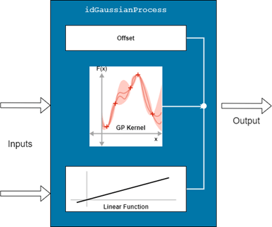
Use an idGaussianProcess object to represent the nonlinear function. Create a GP representation based on the ARD Matern32 kernel. For this model, you do not use the linear model to initialize the model structure. Instead, create the regressors directly using the linearRegressor command.
Kernel = 'ARDMatern32';
GP = idGaussianProcess(Kernel);
MaxLag = 4; % maximum number of delays in each regressor
OutputLags = 1:MaxLag;
InputLags = 0:MaxLag;
Reg = linearRegressor([Output, Inputs],{OutputLags,InputLags,InputLags,InputLags,InputLags})
Reg =
Linear regressors in variables EngineTorque, ThrottlePosition, WastegateValve, EngineSpeed, SparkTiming
       Variables: {'EngineTorque'  'ThrottlePosition'  'WastegateValve'  'EngineSpeed'  'SparkTiming'}
            Lags: {[1 2 3 4]  [0 1 2 3 4]  [0 1 2 3 4]  [0 1 2 3 4]  [0 1 2 3 4]}
     UseAbsolute: [0 0 0 0 0]
    TimeVariable: 't'

  Regressors described by this set
Use the estimation data (eDataD), the regressor set (Reg), and the nonlinear function (GP) in the nlarx command to train the GP-based nonlinear ARX model.
nlarxopt.SearchOptions.MaxIterations = 20;
tic
GPModel = nlarx(eDataD,Reg,GP,nlarxopt)
|=====================================================================================================|
|   ITER   |   FUN VALUE   |  NORM GRAD  |  NORM STEP  | CG TERM |     RHO     |  TRUST RAD  | ACCEPT |
|=====================================================================================================|
|        0 |  -4.31381e+03 |   6.390e+02 |   1.032e+00 |   CONV  |   2.065e+00 |   5.099e+00 |   YES  |
|        1 |  -4.31381e+03 |   6.390e+02 |   5.099e+00 |  EXACT  |  -2.375e+00 |   5.099e+00 |    NO  |
|        2 |  -5.32039e+03 |   8.618e+02 |   2.550e+00 |  EXACT  |   2.711e-01 |   2.550e+00 |   YES  |
|        3 |  -5.34697e+03 |   8.088e+02 |   2.942e-02 |   CONV  |   1.947e+00 |   2.550e+00 |   YES  |
|        4 |  -5.48306e+03 |   7.906e+02 |   5.351e-01 |   CONV  |   5.787e-01 |   2.550e+00 |   YES  |
|        5 |  -5.58226e+03 |   2.694e+02 |   2.963e-01 |   CONV  |   7.755e-01 |   2.550e+00 |   YES  |
|        6 |  -6.01284e+03 |   1.156e+02 |   1.758e+00 |   CONV  |   1.627e+00 |   2.550e+00 |   YES  |
|        7 |  -6.57309e+03 |   8.562e+01 |   2.550e+00 |  BNDRY  |   1.412e+00 |   2.550e+00 |   YES  |
|        8 |  -7.52416e+03 |   4.205e+02 |   5.099e+00 |  BNDRY  |   1.280e+00 |   5.099e+00 |   YES  |
|        9 |  -7.52416e+03 |   4.205e+02 |   1.020e+01 |  EXACT  |  -2.768e-01 |   1.020e+01 |    NO  |
|       10 |  -7.94111e+03 |   1.253e+02 |   5.099e+00 |  BNDRY  |   7.350e-01 |   5.099e+00 |   YES  |
|       11 |  -7.95215e+03 |   5.025e+02 |   1.100e+00 |   CONV  |   2.483e-01 |   5.099e+00 |   YES  |
|       12 |  -7.98119e+03 |   2.517e+02 |   7.176e-02 |   CONV  |   1.508e+00 |   5.099e+00 |   YES  |
|       13 |  -7.99465e+03 |   5.390e+01 |   8.582e-02 |   CONV  |   1.111e+00 |   5.099e+00 |   YES  |
|       14 |  -8.06705e+03 |   6.143e+01 |   3.915e+00 |   CONV  |   9.341e-01 |   5.099e+00 |   YES  |
|       15 |  -8.06705e+03 |   6.143e+01 |   5.099e+00 |  EXACT  |  -1.172e-01 |   5.099e+00 |    NO  |
|       16 |  -8.10383e+03 |   2.499e+02 |   2.550e+00 |  BNDRY  |   3.153e-01 |   2.550e+00 |   YES  |
|       17 |  -8.15516e+03 |   7.926e+01 |   3.375e-01 |   CONV  |   1.513e+00 |   2.550e+00 |   YES  |
|       18 |  -8.15516e+03 |   7.926e+01 |   2.550e+00 |  EXACT  |  -1.237e-01 |   2.550e+00 |    NO  |
|       19 |  -8.18832e+03 |   4.826e+01 |   7.055e-01 |   CONV  |   9.162e-01 |   1.275e+00 |   YES  |

|=====================================================================================================|
|   ITER   |   FUN VALUE   |  NORM GRAD  |  NORM STEP  | CG TERM |     RHO     |  TRUST RAD  | ACCEPT |
|=====================================================================================================|
|       20 |  -8.20116e+03 |   2.206e+01 |   7.437e-01 |   CONV  |   1.322e+00 |   1.275e+00 |   YES  |
|       21 |  -8.21145e+03 |   3.409e+01 |   1.037e+00 |   CONV  |   1.281e+00 |   1.275e+00 |   YES  |
|       22 |  -8.21145e+03 |   3.409e+01 |   2.550e+00 |  BNDRY  |  -3.629e+00 |   2.550e+00 |    NO  |
|       23 |  -8.21145e+03 |   3.409e+01 |   1.127e+00 |   CONV  |  -5.062e-01 |   1.275e+00 |    NO  |
|       24 |  -8.22017e+03 |   3.439e+01 |   5.506e-01 |   CONV  |   8.055e-01 |   6.374e-01 |   YES  |
|       25 |  -8.22136e+03 |   2.039e+01 |   3.785e-02 |   CONV  |   1.832e+00 |   1.275e+00 |   YES  |
|       26 |  -8.22597e+03 |   5.089e+01 |   3.345e-01 |   CONV  |   1.068e+00 |   1.275e+00 |   YES  |
|       27 |  -8.22597e+03 |   5.089e+01 |   1.275e+00 |  EXACT  |  -5.419e-01 |   1.275e+00 |    NO  |
|       28 |  -8.22626e+03 |   3.609e+01 |   5.768e-03 |   CONV  |   1.734e+00 |   6.374e-01 |   YES  |
|       29 |  -8.22662e+03 |   7.013e+00 |   1.710e-02 |   CONV  |   9.861e-01 |   6.374e-01 |   YES  |
|       30 |  -8.23051e+03 |   2.482e+01 |   6.374e-01 |  EXACT  |   1.772e-01 |   6.374e-01 |   YES  |
|       31 |  -8.23420e+03 |   9.671e+00 |   6.374e-01 |  BNDRY  |   8.748e-01 |   6.374e-01 |   YES  |
|       32 |  -8.23669e+03 |   1.880e+01 |   7.042e-01 |   CONV  |   1.155e+00 |   1.275e+00 |   YES  |
|       33 |  -8.23669e+03 |   1.880e+01 |   1.275e+00 |  EXACT  |  -1.068e+00 |   1.275e+00 |    NO  |
|       34 |  -8.23828e+03 |   1.615e+01 |   2.225e-01 |   CONV  |   8.991e-01 |   6.374e-01 |   YES  |
|       35 |  -8.23847e+03 |   1.237e+01 |   1.484e-02 |   CONV  |   1.863e+00 |   6.374e-01 |   YES  |
|       36 |  -8.24006e+03 |   8.779e+00 |   3.812e-01 |   CONV  |   1.066e+00 |   6.374e-01 |   YES  |
|       37 |  -8.24006e+03 |   8.779e+00 |   6.374e-01 |  BNDRY  |  -6.237e-01 |   6.374e-01 |    NO  |
|       38 |  -8.24105e+03 |   5.596e+00 |   3.187e-01 |  BNDRY  |   1.046e+00 |   3.187e-01 |   YES  |
|       39 |  -8.24105e+03 |   5.596e+00 |   6.374e-01 |  EXACT  |  -2.335e-01 |   6.374e-01 |    NO  |

|=====================================================================================================|
|   ITER   |   FUN VALUE   |  NORM GRAD  |  NORM STEP  | CG TERM |     RHO     |  TRUST RAD  | ACCEPT |
|=====================================================================================================|
|       40 |  -8.24212e+03 |   6.079e+00 |   3.187e-01 |  BNDRY  |   1.096e+00 |   3.187e-01 |   YES  |
|       41 |  -8.24340e+03 |   3.426e+00 |   6.374e-01 |  BNDRY  |   1.199e+00 |   6.374e-01 |   YES  |
|       42 |  -8.24405e+03 |   6.151e+00 |   6.331e-01 |   CONV  |   1.277e+00 |   1.275e+00 |   YES  |
|       43 |  -8.24424e+03 |   2.985e+00 |   3.413e-02 |   CONV  |   1.661e+00 |   1.275e+00 |   YES  |
|       44 |  -8.24468e+03 |   6.391e+00 |   1.814e-01 |   CONV  |   1.056e+00 |   1.275e+00 |   YES  |
|       45 |  -8.24468e+03 |   6.391e+00 |   1.275e+00 |  EXACT  |  -3.821e-01 |   1.275e+00 |    NO  |
|       46 |  -8.24468e+03 |   6.391e+00 |   6.374e-01 |  BNDRY  |  -4.656e+00 |   6.374e-01 |    NO  |
|       47 |  -8.24536e+03 |   7.616e+00 |   3.187e-01 |  BNDRY  |   1.039e+00 |   3.187e-01 |   YES  |
|       48 |  -8.24536e+03 |   7.616e+00 |   6.374e-01 |  EXACT  |  -2.959e-01 |   6.374e-01 |    NO  |
|       49 |  -8.24560e+03 |   8.910e+00 |   5.566e-02 |   CONV  |   1.435e+00 |   3.187e-01 |   YES  |
|       50 |  -8.24562e+03 |   1.954e+00 |   3.145e-03 |   CONV  |   1.250e+00 |   3.187e-01 |   YES  |
|       51 |  -8.24630e+03 |   3.507e+00 |   3.187e-01 |  BNDRY  |   1.029e+00 |   3.187e-01 |   YES  |
|       52 |  -8.24630e+03 |   3.507e+00 |   6.374e-01 |  EXACT  |  -1.048e-01 |   6.374e-01 |    NO  |
|       53 |  -8.24682e+03 |   2.473e+00 |   3.187e-01 |  BNDRY  |   9.019e-01 |   3.187e-01 |   YES  |
|       54 |  -8.24734e+03 |   4.631e+00 |   6.374e-01 |  BNDRY  |   9.942e-01 |   6.374e-01 |   YES  |
|       55 |  -8.24745e+03 |   2.650e+00 |   7.860e-02 |   CONV  |   9.903e-01 |   1.275e+00 |   YES  |
|       56 |  -8.24755e+03 |   7.431e+00 |   3.602e-01 |   CONV  |   7.622e-01 |   1.275e+00 |   YES  |
|       57 |  -8.24756e+03 |   5.763e+00 |   6.981e-04 |   CONV  |   1.816e+00 |   1.275e+00 |   YES  |
|       58 |  -8.24762e+03 |   1.269e+00 |   1.945e-02 |   CONV  |   1.462e+00 |   1.275e+00 |   YES  |
|       59 |  -8.24791e+03 |   2.822e+00 |   5.737e-01 |   CONV  |   1.040e+00 |   1.275e+00 |   YES  |

|=====================================================================================================|
|   ITER   |   FUN VALUE   |  NORM GRAD  |  NORM STEP  | CG TERM |     RHO     |  TRUST RAD  | ACCEPT |
|=====================================================================================================|
|       60 |  -8.24791e+03 |   2.822e+00 |   1.275e+00 |  EXACT  |  -3.889e-01 |   1.275e+00 |    NO  |
|       61 |  -8.24812e+03 |   6.709e+00 |   1.927e-01 |   CONV  |   8.686e-01 |   6.374e-01 |   YES  |
|       62 |  -8.24816e+03 |   5.054e+00 |   6.719e-03 |   CONV  |   1.864e+00 |   6.374e-01 |   YES  |
|       63 |  -8.24836e+03 |   1.373e+00 |   8.133e-02 |   CONV  |   1.078e+00 |   6.374e-01 |   YES  |
|       64 |  -8.24871e+03 |   1.862e+00 |   6.374e-01 |  BNDRY  |   1.001e+00 |   6.374e-01 |   YES  |
|       65 |  -8.24871e+03 |   1.862e+00 |   1.275e+00 |  EXACT  |  -6.497e-01 |   1.275e+00 |    NO  |
|       66 |  -8.24900e+03 |   1.250e+00 |   6.374e-01 |  BNDRY  |   1.147e+00 |   6.374e-01 |   YES  |
|       67 |  -8.24913e+03 |   1.557e+00 |   6.299e-01 |   CONV  |   1.117e+00 |   1.275e+00 |   YES  |
|       68 |  -8.24915e+03 |   3.209e+00 |   1.329e-01 |   CONV  |   2.260e-01 |   1.275e+00 |   YES  |
|       69 |  -8.24919e+03 |   1.778e+00 |   1.120e-02 |   CONV  |   1.726e+00 |   1.275e+00 |   YES  |
|       70 |  -8.24935e+03 |   9.370e-01 |   1.813e-01 |   CONV  |   9.970e-01 |   1.275e+00 |   YES  |
|       71 |  -8.24935e+03 |   9.463e-01 |   1.069e-02 |   CONV  |   1.078e+00 |   1.275e+00 |   YES  |
|       72 |  -8.24936e+03 |   1.432e+00 |   7.025e-02 |   CONV  |   6.170e-01 |   1.275e+00 |   YES  |
|       73 |  -8.24936e+03 |   1.177e+00 |   4.733e-03 |   CONV  |   1.613e+00 |   1.275e+00 |   YES  |
|       74 |  -8.24937e+03 |   8.417e-01 |   2.061e-02 |   CONV  |   1.085e+00 |   1.275e+00 |   YES  |
|       75 |  -8.24937e+03 |   9.137e-01 |   1.703e-03 |   CONV  |   1.779e+00 |   1.275e+00 |   YES  |
|       76 |  -8.24937e+03 |   9.104e-01 |   5.393e-05 |   CONV  |   1.998e+00 |   1.275e+00 |   YES  |
|       77 |  -8.24964e+03 |   3.007e+00 |   1.250e+00 |   CONV  |   1.228e+00 |   1.275e+00 |   YES  |
|       78 |  -8.24964e+03 |   6.524e-01 |   1.298e-03 |   CONV  |   1.014e+00 |   2.550e+00 |   YES  |
|       79 |  -8.24964e+03 |   6.524e-01 |   2.550e+00 |  EXACT  |  -4.133e-02 |   2.550e+00 |    NO  |

|=====================================================================================================|
|   ITER   |   FUN VALUE   |  NORM GRAD  |  NORM STEP  | CG TERM |     RHO     |  TRUST RAD  | ACCEPT |
|=====================================================================================================|
|       80 |  -8.24964e+03 |   6.524e-01 |   1.275e+00 |  EXACT  |  -1.106e+00 |   1.275e+00 |    NO  |
|       81 |  -8.24969e+03 |   6.269e-01 |   1.967e-01 |   CONV  |   1.008e+00 |   6.374e-01 |   YES  |
|       82 |  -8.24969e+03 |   6.269e-01 |   6.374e-01 |  EXACT  |  -2.622e-01 |   6.374e-01 |    NO  |
|       83 |  -8.24970e+03 |   5.479e-01 |   1.989e-02 |   CONV  |   1.447e+00 |   3.187e-01 |   YES  |
|       84 |  -8.24972e+03 |   1.283e+00 |   2.616e-01 |   CONV  |   1.158e+00 |   3.187e-01 |   YES  |
|       85 |  -8.24973e+03 |   1.159e+00 |   1.618e-02 |   CONV  |   1.333e+00 |   6.374e-01 |   YES  |
|       86 |  -8.24973e+03 |   1.159e+00 |   6.374e-01 |  EXACT  |  -1.149e+00 |   6.374e-01 |    NO  |
|       87 |  -8.24974e+03 |   1.998e-01 |   2.945e-02 |   CONV  |   1.024e+00 |   3.187e-01 |   YES  |
|       88 |  -8.24977e+03 |   2.238e+00 |   3.187e-01 |  BNDRY  |   8.203e-01 |   3.187e-01 |   YES  |
|       89 |  -8.24977e+03 |   3.604e-01 |   8.787e-04 |   CONV  |   1.007e+00 |   6.374e-01 |   YES  |
|       90 |  -8.24977e+03 |   3.604e-01 |   6.374e-01 |  EXACT  |  -3.169e-02 |   6.374e-01 |    NO  |
|       91 |  -8.24980e+03 |   5.040e-01 |   3.187e-01 |  BNDRY  |   9.506e-01 |   3.187e-01 |   YES  |
|       92 |  -8.24980e+03 |   1.359e-01 |   6.158e-02 |   CONV  |   1.030e+00 |   6.374e-01 |   YES  |
|       93 |  -8.24980e+03 |   1.359e-01 |   6.374e-01 |  EXACT  |  -1.369e+00 |   6.374e-01 |    NO  |
|       94 |  -8.24981e+03 |   6.139e-01 |   3.187e-01 |  BNDRY  |   1.044e+00 |   3.187e-01 |   YES  |
|       95 |  -8.24981e+03 |   6.139e-01 |   6.374e-01 |  EXACT  |  -2.588e-01 |   6.374e-01 |    NO  |
|       96 |  -8.24981e+03 |   6.139e-01 |   2.736e-02 |   CONV  |  -1.110e-01 |   3.187e-01 |    NO  |
|       97 |  -8.24982e+03 |   8.049e-02 |   1.321e-02 |   CONV  |   1.006e+00 |   1.593e-01 |   YES  |
|       98 |  -8.24982e+03 |   7.326e-01 |   1.593e-01 |  BNDRY  |   4.450e-01 |   1.593e-01 |   YES  |
|       99 |  -8.24982e+03 |   9.770e-02 |   8.839e-03 |   CONV  |   1.048e+00 |   1.593e-01 |   YES  |

|=====================================================================================================|
|   ITER   |   FUN VALUE   |  NORM GRAD  |  NORM STEP  | CG TERM |     RHO     |  TRUST RAD  | ACCEPT |
|=====================================================================================================|
|      100 |  -8.24983e+03 |   1.482e-01 |   1.593e-01 |  BNDRY  |   1.086e+00 |   1.593e-01 |   YES  |
|      101 |  -8.24983e+03 |   1.482e-01 |   3.187e-01 |  BNDRY  |  -4.454e+00 |   3.187e-01 |    NO  |
|      102 |  -8.24983e+03 |   8.207e-02 |   1.593e-01 |  BNDRY  |   1.101e+00 |   1.593e-01 |   YES  |
|      103 |  -8.24984e+03 |   1.169e-01 |   3.187e-01 |  BNDRY  |   9.531e-01 |   3.187e-01 |   YES  |
|      104 |  -8.24984e+03 |   5.347e-02 |   8.441e-02 |   CONV  |   1.037e+00 |   6.374e-01 |   YES  |
|      105 |  -8.24985e+03 |   5.682e-02 |   6.374e-01 |  BNDRY  |   1.356e+00 |   6.374e-01 |   YES  |
|      106 |  -8.24986e+03 |   6.853e-02 |   1.254e+00 |   CONV  |   1.380e+00 |   1.275e+00 |   YES  |
|      107 |  -8.24986e+03 |   2.750e-02 |   8.298e-02 |   CONV  |   1.086e+00 |   2.550e+00 |   YES  |
|      108 |  -8.24987e+03 |   9.546e-03 |   1.306e+00 |   CONV  |   1.484e+00 |   2.550e+00 |   YES  |
|      109 |  -8.24987e+03 |   1.305e-02 |   1.548e+00 |   CONV  |   1.451e+00 |   2.550e+00 |   YES  |
|      110 |  -8.24987e+03 |   7.745e-03 |   1.654e+00 |   CONV  |   1.464e+00 |   2.550e+00 |   YES  |
|      111 |  -8.24988e+03 |   3.639e-03 |   1.807e+00 |   CONV  |   1.458e+00 |   2.550e+00 |   YES  |
|      112 |  -8.24988e+03 |   3.351e-03 |   1.929e+00 |   CONV  |   1.456e+00 |   2.550e+00 |   YES  |
|      113 |  -8.24988e+03 |   1.193e-03 |   2.035e+00 |   CONV  |   1.452e+00 |   2.550e+00 |   YES  |
|      114 |  -8.24988e+03 |   1.229e-03 |   2.113e+00 |   CONV  |   1.449e+00 |   2.550e+00 |   YES  |
|      115 |  -8.24988e+03 |   4.007e-04 |   2.167e+00 |   CONV  |   1.446e+00 |   5.099e+00 |   YES  |

         Infinity norm of the final gradient = 4.007e-04
              Two norm of the final step     = 2.167e+00, TolX   = 1.000e-12
Relative infinity norm of the final gradient = 7.981e-07, TolFun = 1.000e-06
EXIT: Local minimum found.

GPModel =

Nonlinear ARX model with 1 output and 4 inputs
  Inputs: ThrottlePosition, WastegateValve, EngineSpeed, SparkTiming
  Outputs: EngineTorque

Regressors:
  Linear regressors in variables EngineTorque, ThrottlePosition, WastegateValve, EngineSpeed, SparkTiming
  List of all regressors

Output function: Gaussian process function using a ARDMatern32 kernel
Sample time: 1 seconds

Status:
Estimated using NLARX on time domain data "eDataD".
Fit to estimation data: 99.97% (simulation focus)
FPE: 2.672e-05, MSE: 5.032e-05

Model Properties
toc
Elapsed time is 665.189346 seconds.
Validate the model.
subplot(211)
compare(eDataD,GPModel)  % compare against estimation data
title('GP Model: Comparison to Estimation Data')

subplot(212)

compare(vDataD,GPModel)  % compare against validation data
title('Comparison to Validation Data')
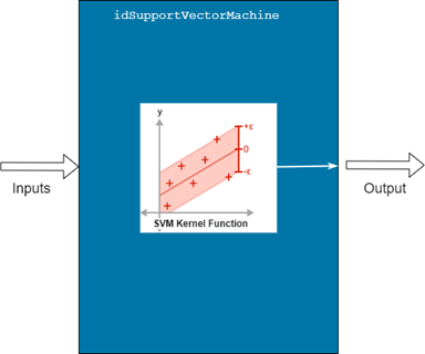
Support Vector Machine (SVM) Model
As a third option, build an SVM-based nonlinear ARX model.

Unlike the GP- and sigmoid-network-based representations, SVM models do not provide a parallel connection of separate linear and nonlinear functions. Use an idSupportVectorMachine object to represent the function.
% Nonlinear function configuration
Kernel = 'Gaussian';
EpsilonMargin = 3.7204e-5;
BoxConstraint = 5.2530;
SVMFcn = idSupportVectorMachine(Kernel);
SVMFcn.BoxConstraint = BoxConstraint;
SVMFcn.EpsilonMargin = EpsilonMargin;

% Regressor configuration
MaxLag = 1;
OutputLags = 1:MaxLag;
InputLags = 0:MaxLag;
Reg2 = linearRegressor([Output, Inputs],{OutputLags,InputLags,InputLags,InputLags,InputLags});
Use the data (eDataD), the regressor set (Reg2), and the nonlinear function (SVMFcn) in the nlarx command to train the SVM based nonlinear ARX model. Note that unlike the GP- and sigmoid-network-based models, SVM-based models do not support a simulation focus. The model must be trained with a prediction focus. The validation is still based on comparing the simulated response of the trained model.
nlarxopt.Focus = 'prediction';
nlarxopt.SearchOptions.MaxIterations = 100;

tic
SVMModel = nlarx(eDataD,Reg2,SVMFcn,nlarxopt)
SVMModel = Nonlinear ARX model with 1 output and 4 inputs Inputs: ThrottlePosition, WastegateValve, EngineSpeed, SparkTiming Outputs: EngineTorque Regressors: Linear regressors in variables EngineTorque, ThrottlePosition, WastegateValve, EngineSpeed, SparkTiming List of all regressors Output function: Support Vector Machine function using a Gaussian kernel Sample time: 1 seconds Status: Estimated using NLARX on time domain data "eDataD". Fit to estimation data: 98.44% (prediction focus) FPE: 4.136, MSE: 0.1445 Model Properties
toc
Elapsed time is 34.983571 seconds.
Validate the model.
subplot(211)
compare(eDataD,SVMModel)  % compare against estimation data
title('SVM Model: Comparison to Estimation Data')

subplot(212)
compare(vDataD,SVMModel)  % compare against validation data
title('Comparison to Validation Data (Downsampled)')
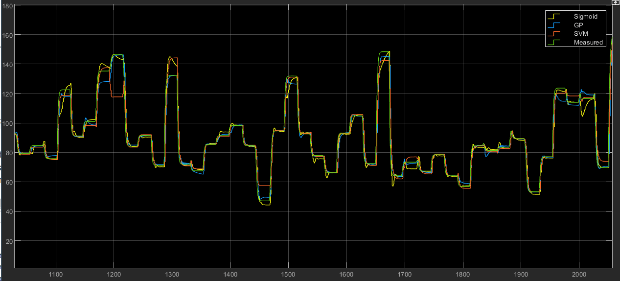
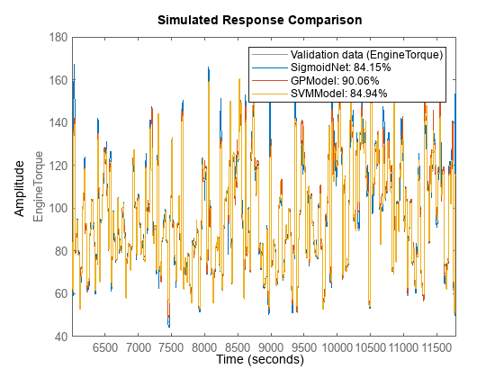
Result Validation
In this example, you create three different types of nonlinear ARX models based on the nature of the function that maps the regressors to the output. All three models show comparably good fits to the validation data.
clf
compare(vDataD,SigmoidNet,GPModel,SVMModel)
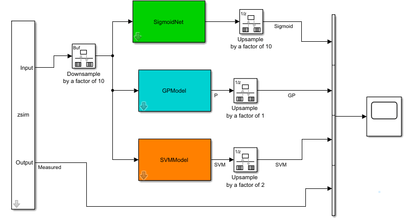
However, note that the training and validation has been performed on the downsampled datasets. If your application requires running the nonlinear ARX model at the original rate of 10 Hz, you can do so in Simulink® by using the rate transition blocks at the input/output ports of the nonlinear ARX Model block.
% Create an iddata representation of the data in vData to feed the signals to the Simulink
% model using an IDDATA Source block.
zsim = iddata(vData,InputName=Inputs,OutputName=Output);
zsim.Tstart = 0;

% Open the simulation model and simulate it using zsim as the source of input data.
mdl = 'nlarx_simulator';
open_system(mdl)

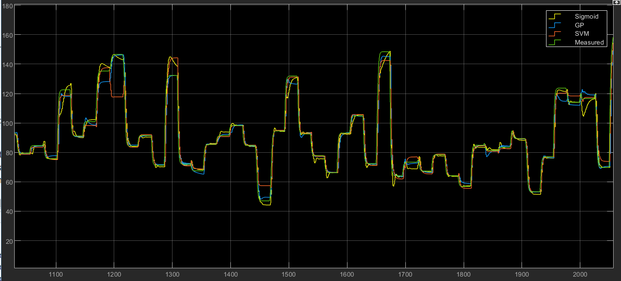
sim(mdl);
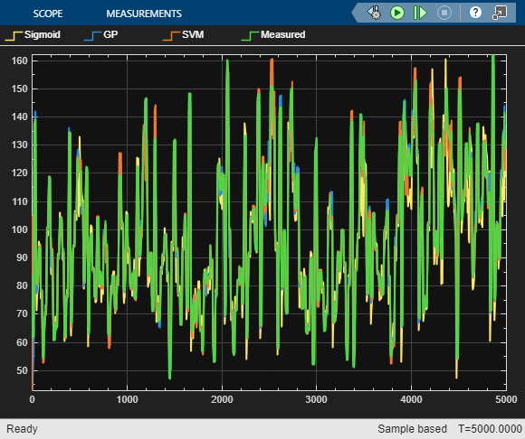
After the initial transients owing to mismatching initial conditions, all the three models are able to emulate the measured engine torque with high accuracy. The nonlinear ARX models thus created can be used as a data-based proxy for the original high-fidelity system for use in resource-constrained environments.