Estimating Transfer Function Models for a Boost Converter
This example shows how to estimate a transfer function from frequency response data. You use Simulink® Control Design™ to collect frequency response data from a Simulink model and the tfest command to estimate a transfer function from the measured data. To run the example with previously saved frequency response data start from the Estimating a Transfer Function section.
Boost Converter
Open the Simulink model.
mdl = 'iddemo_boost_converter';
open_system(mdl);
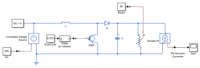
The model is of a Boost Converter circuit that converts a DC voltage to another DC voltage (typically a higher voltage) by controlled chopping or switching of the source voltage. In this model an IGBT driven by a PWM signal is used for switching.
For this example we are interested in the transfer function from the PWM duty cycle set-point to the load voltage, Uout.
Collect Frequency Response Data
We use the frestimate command to perturb the duty cycle set-point with sinusoids of different frequencies and log the resulting load voltage. From these we find how the system modifies the magnitude and phase of the injected sinusoids giving us discrete points on the frequency response.
Using frestimate requires two preliminary steps
Specifying the frequency response input and output points
Defining the sinusoids to inject at the input point
The frequency response input and output points are created using the linio command and for this example are the outputs of the DutyCycle and Voltage Measurement blocks.
ios = [...
    linio([mdl,'/DutyCycle'],1,'input'); ...
    linio([mdl,'/PS-Simulink Converter'],1,'output')];
We use the frest.Sinestream command to define the sinusoids to inject at the input point. We are interested in the frequency range 200 to 20k rad/s, and want to perturb the duty cycle by 0.03.
f = logspace(log10(200),log10(20000),10);
in = frest.Sinestream('Frequency',f,'Amplitude',0.03);
The simulation time required to simulate the model with this sine-stream signal is determined using the getSimulationTime command and as we know the simulation end time used by the model we can get an idea of how much longer the sine-stream simulation will take over simply running the model.
getSimulationTime(in)/0.02
ans =

   15.5933
We use the defined inputs and sine-stream with frestimate to compute discrete points on the frequency response.
[sysData,simlog] = frestimate(mdl,ios,in);
bopt               = bodeoptions;
bopt.Grid          = 'on';
bopt.PhaseMatching = 'on';
figure, bode(sysData,'*r',bopt)
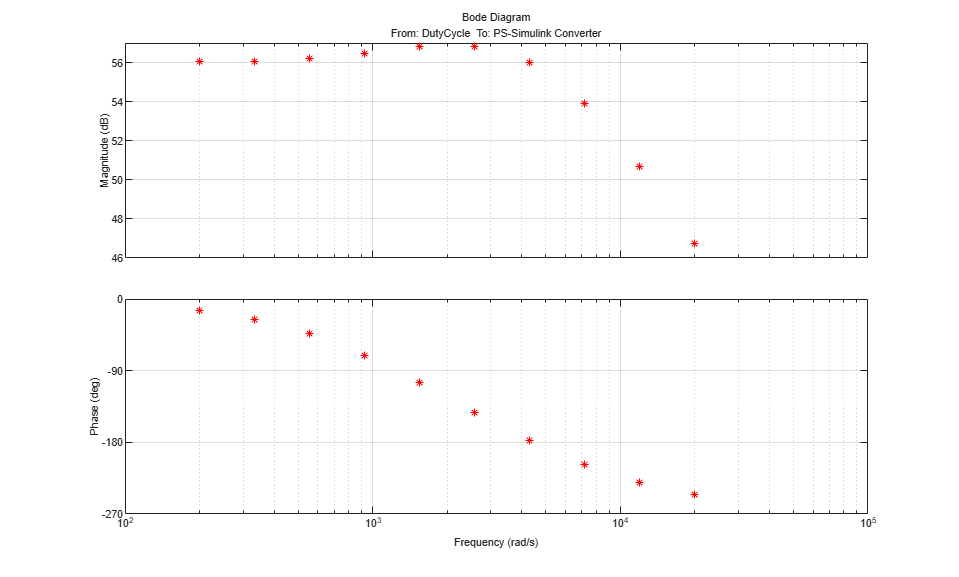
The Bode response shows a system with a 56db gain, some minor resonance around 2500 rad/s and a high frequency roll off of around 20 db/decade matching what we would expect for this circuit.
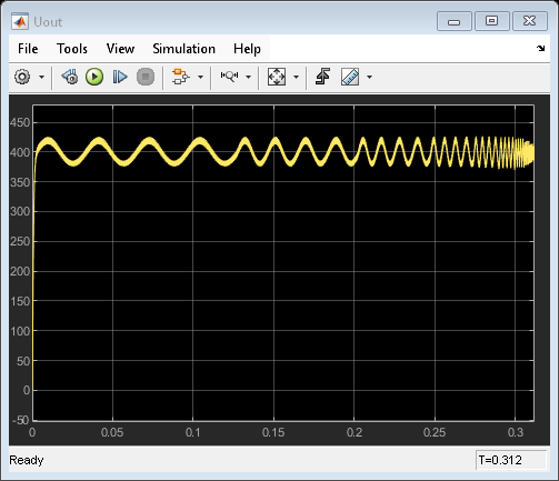
The frest.simView command allows us to inspect the frestimate process showing the injected signal, measured output, and frequency response in one graphical interface.
frest.simView(simlog,in,sysData);

The figure shows the model response to injected sinusoids and the FFT of the model response. Notice that the injected sinusoids result in signals with a dominant frequency and limited harmonics indicating a linear model and successful frequency response data collection.
Estimating a Transfer Function
In the previous step we collected frequency response data. This data describes the system as discrete frequency points and we now fit a transfer function to the data.
We generated the frequency response data using Simulink Control Design, if Simulink Control Design is not installed use the following command to load the saved frequency response data
load iddemo_boostconverter_data
Inspecting the frequency response data we expect that the system can be described by a second order system.
sysA = tfest(sysData,2)
figure, bode(sysData,'r*',sysA,bopt)
sysA =

  From input "DutyCycle" to output "PS-Simulink Converter":
  -4.456e06 s + 6.175e09
  -----------------------
  s^2 + 6995 s + 9.834e06

Continuous-time identified transfer function.

Parameterization:
   Number of poles: 2   Number of zeros: 1
   Number of free coefficients: 4
   Use "tfdata", "getpvec", "getcov" for parameters and their uncertainties.

Status:
Estimated using TFEST on frequency response data "sysData".
Fit to estimation data: 98.04%
FPE: 281.4, MSE: 120.6
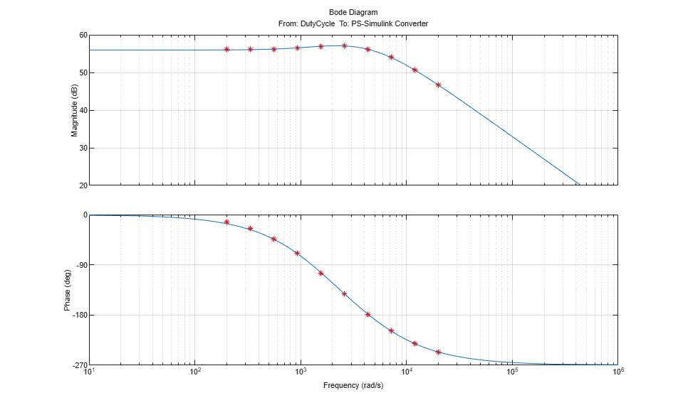
The estimated transfer function is accurate over the provided frequency range.
bdclose(mdl)
You can also select a web site from the following list:
Americas
- América Latina (Español)
- Canada (English)
- United States (English)
Europe
- Belgium (English)
- Denmark (English)
- Deutschland (Deutsch)
- España (Español)
- Finland (English)
- France (Français)
- Ireland (English)
- Italia (Italiano)
- Luxembourg (English)
- Netherlands (English)
- Norway (English)
- Österreich (Deutsch)
- Portugal (English)
- Sweden (English)
- Switzerland
- United Kingdom (English)