Cylinder Linearization
This example shows how you can linearize a Simscape™ hydro-mechanical system model to check stability of an open-loop system around an operating point. This example uses the Simulink Control Design™ Frequency Response Estimator block to perform a frequency response estimation experiment and store the data for later estimation offline.
Model
The model contains a plant, Tandem Primary cylinder in an open-loop configuration. The Frequency Response Estimator block accepts the input signal u. It feeds a sum of input signal and a Sinestream perturbation into the Simulink-PS converter block. The Simulink-PS converter block injects the sum of the operating point input and the sinestream to the Tandem Primary Cylinder subsystem.

Offline Frequency Response Estimation
Frequency response describes the steady state response of a system to a sinusoidal input signal. If the system is linear G(s), the output signal is a sine wave of the same frequency with a different magnitude and a phase shift. A frequency response data (frd) model that stores frequency response information at multiple frequencies is useful for tasks such as analyzing plant dynamics, understanding open-loop and closed-loop stability, validating linearization results, designing a control system, and estimating a parametric model.
You can use the Simulink Control Design™ frestimate command or use the Model Linearizer app to run a simulation with some perturbation signals on the Simscape model. Afterwards, the plant frequency responses are estimated offline based on the collected experiment data. This approach is called offline estimation.
When generating data from simulating the model, it is important that the physics should not encounter non-linearities like friction, saturation, hardstop, and switching. This is required for the correct frequency response estimation for the system of interest.
Hydro-mechanical System Stability Estimation Using Sinestream Mode
The model contains the Frequency Response Estimator block in the control signal + perturbation output configuration setting. You can use the start/stop signal to start and stop a frequency response estimation experiment in this configuration setting.
During the experiment, when the Experiment Mode is in Sinestream setting, the block injects sinusoidal signals into to the Simulink-PS converter block one frequency after another, from the lowest to the highest.
Frequency Response Estimator block has a data outport that allows you to log a time series experiment data from simulation. You can process that data set offline with the frestimate command to generate an frd object.
Frequency Response Estimator block also has an frd outport that allows you to log the frequency response data from simulation. You can process that data set offline with the frd command to generate an frd object.
sim('sscv_cylinder_linearization')
sysEstimFRD1 = frestimate(dataTimeSeries,omega,'rad/s');
sysEstimFRD2  = frd(dataFreqDomain,omega);
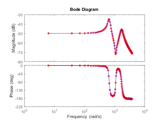
You can use generated frd objects to create the bode plot for the system. The generated bode plot will be same for the generated frd objects, sysEstimFRD1 and sysEstimFRD2.
figure;
bode(sysEstimFRD1, 'r*')
hold;
Current plot held
bode(sysEstimFRD2,'b')
You can use the System Identification Toolbox™ pem or ssest command to identify a state-space model fitting the frd object. The sysEstimFRD2 frd object will create a continuous state-space model, however sysEstimFRD1 frd object will create a discrete state-space model.
sysEstimIdentFRD1 = n4sid(sysEstimFRD1,5, 'Ts', sysEstimFRD1.Ts);
sysEstimIdentFRD2 = n4sid(sysEstimFRD2,5);
You can use the System Identification Toolbox compare command to check the fit quality between the estimated state-space model, sysEstimIdentFRD1 or sysEstimIdentFRD2 and the generated frd object, sysEstimFRD1 or sysEstimFRD2 respectively.
figure;
compare(sysEstimFRD1,sysEstimIdentFRD1)

You can use the Control System Toolbox™ pole command to estimate the poles of the system using the identified state-space model. If the poles are on the left side of the s-plane for the continuous state-space model, sysEstimIdentFRD2, then the open-loop hydro-mechanical system of interest is a stable system around the selected operating point.
poles = pole(sysEstimIdentFRD2)
poles = 5×1 complex
103 ×

  -0.0882 + 1.6894i
  -0.0882 - 1.6894i
  -0.0329 + 0.6556i
  -0.0329 - 0.6556i
  -1.1461 + 0.0000i
Similarly, for the discrete state-space model, sysEstimIdentFRD1, if the poles lie within the unit circle then the open-loop hydro-mechanical system of interest is a stable system around the selected operating point.
poles = pole(sysEstimIdentFRD1)
poles = 5×1 complex

   0.9773 + 0.1673i
   0.9773 - 0.1673i
   0.9948 + 0.0656i
   0.9948 - 0.0656i
   0.9056 + 0.0000i
magnitude = abs(poles)
magnitude = 5×1

    0.9915
    0.9915
    0.9969
    0.9969
    0.9056