Tune Particle Swarm Optimization Process
This example shows how to optimize using the particleswarm solver. The particle swarm algorithm moves a population of particles called a swarm toward a minimum of an objective function. The velocity of each particle in the swarm changes according to three factors:
The effect of inertia (
InertiaRangeoption)An attraction to the best location the particle has visited (
SelfAdjustmentWeightoption)An attraction to the best location among neighboring particles (
SocialAdjustmentWeightoption)
This example shows some effects of changing particle swarm options.
When to Modify Options
Often, particleswarm finds a good solution when using its default options. For example, it optimizes rastriginsfcn well with the default options. This function has many local minima, and a global minimum of 0 at the point [0,0].
rng default % for reproducibility
[x,fval,exitflag,output] = particleswarm(@rastriginsfcn,2);
Optimization ended: relative change in the objective value
over the last OPTIONS.MaxStallIterations iterations is less than OPTIONS.FunctionTolerance.
formatstring = "particleswarm reached the value %f using %d function evaluations.\n";
fprintf(formatstring,fval,output.funccount)
particleswarm reached the value 0.000000 using 2560 function evaluations.
For this function, you know the optimal objective value, so you know that the solver found it. But what if you do not know the solution? One way to evaluate the solution quality is to rerun the solver.
[x,fval,exitflag,output] = particleswarm(@rastriginsfcn,2);
Optimization ended: relative change in the objective value
over the last OPTIONS.MaxStallIterations iterations is less than OPTIONS.FunctionTolerance.
fprintf(formatstring,fval,output.funccount)
particleswarm reached the value 0.000000 using 1480 function evaluations.
Both the solution and the number of function evaluations are similar to the previous run. This suggests that the solver is not having difficulty arriving at a solution.
Difficult Objective Function Using Default Parameters
The Rosenbrock function is well known to be a difficult function to optimize. This example uses a multidimensional version of the Rosenbrock function. The function has a minimum value of 0 at the point [1,1,1,...].
rng default % for reproducibility
nvars = 6; % choose any even value for nvars
fun = @multirosenbrock;
[x,fval,exitflag,output] = particleswarm(fun,nvars);
Optimization ended: relative change in the objective value
over the last OPTIONS.MaxStallIterations iterations is less than OPTIONS.FunctionTolerance.
fprintf(formatstring,fval,output.funccount)
particleswarm reached the value 3106.436648 using 12960 function evaluations.
The solver did not find a very good solution.
Bound the Search Space
Try bounding the space to help the solver locate a good point.
lb = -10*ones(1,nvars);
ub = -lb;
[xbounded,fvalbounded,exitflagbounded,outputbounded] = particleswarm(fun,nvars,lb,ub);
Optimization ended: relative change in the objective value
over the last OPTIONS.MaxStallIterations iterations is less than OPTIONS.FunctionTolerance.
fprintf(formatstring,fvalbounded,outputbounded.funccount)
particleswarm reached the value 0.000006 using 71160 function evaluations.
The solver found a much better solution. But it took a very large number of function evaluations to do so.
Change Options
Perhaps the solver would converge faster if it paid more attention to the best neighbor in the entire space, rather than some smaller neighborhood.
options = optimoptions("particleswarm",MinNeighborsFraction=1);
[xn,fvaln,exitflagn,outputn] = particleswarm(fun,nvars,lb,ub,options);
Optimization ended: relative change in the objective value over the last OPTIONS.MaxStallIterations iterations is less than OPTIONS.FunctionTolerance.
fprintf(formatstring,fvaln,outputn.funccount)
particleswarm reached the value 0.000462 using 30180 function evaluations.
While the solver took fewer function evaluations, it is unclear if this was due to randomness or to a better option setting.
Perhaps you should raise the SelfAdjustmentWeight option.
options.SelfAdjustmentWeight = 1.9; [xn2,fvaln2,exitflagn2,outputn2] = particleswarm(fun,nvars,lb,ub,options);
Optimization ended: relative change in the objective value
over the last OPTIONS.MaxStallIterations iterations is less than OPTIONS.FunctionTolerance.
fprintf(formatstring,fvaln2,outputn2.funccount)
particleswarm reached the value 0.000074 using 18780 function evaluations.
This time particleswarm took even fewer function evaluations. Is this improvement due to randomness, or are the option settings really worthwhile? Rerun the solver and look at the number of function evaluations.
[xn3,fvaln3,exitflagn3,outputn3] = particleswarm(fun,nvars,lb,ub,options);
Optimization ended: relative change in the objective value
over the last OPTIONS.MaxStallIterations iterations is less than OPTIONS.FunctionTolerance.
fprintf(formatstring,fvaln3,outputn3.funccount)
particleswarm reached the value 0.157026 using 53040 function evaluations.
This time the number of function evaluations increased. Apparently, this SelfAdjustmentWeight setting does not necessarily improve performance.
Provide an Initial Point
Perhaps particleswarm would do better if it started from a known point that is not too far from the solution. Try the origin. Give a few individuals at the same initial point. Their random velocities ensure that they do not remain together.
x0 = zeros(20,6); % set 20 individuals as row vectors options.InitialSwarmMatrix = x0; % the rest of the swarm is random [xn3,fvaln3,exitflagn3,outputn3] = particleswarm(fun,nvars,lb,ub,options);
Optimization ended: relative change in the objective value
over the last OPTIONS.MaxStallIterations iterations is less than OPTIONS.FunctionTolerance.
fprintf(formatstring,fvaln3,outputn3.funccount)
particleswarm reached the value 0.039015 using 32100 function evaluations.
The number of function evaluations decreased again.
Vectorize for Speed
The multirosenbrock function allows for vectorized function evaluation. This means that it can simultaneously evaluate the objective function for all particles in the swarm. This usually speeds up the solver considerably.
rng default % do a fair comparison options.UseVectorized = true; tic [xv,fvalv,exitflagv,outputv] = particleswarm(fun,nvars,lb,ub,options);
Optimization ended: relative change in the objective value
over the last OPTIONS.MaxStallIterations iterations is less than OPTIONS.FunctionTolerance.
toc
Elapsed time is 0.094274 seconds.
options.UseVectorized = false;
rng default
tic
[xnv,fvalnv,exitflagnv,outputnv] = particleswarm(fun,nvars,lb,ub,options);
Optimization ended: relative change in the objective value over the last OPTIONS.MaxStallIterations iterations is less than OPTIONS.FunctionTolerance.
toc
Elapsed time is 0.158168 seconds.
The vectorized calculation took about half the time of the serial calculation.
Plot Function
You can view the progress of the solver using a plot function.
options = optimoptions(options,PlotFcn=@pswplotbestf);
rng default
[x,fval,exitflag,output] = particleswarm(fun,nvars,lb,ub,options);
Optimization ended: relative change in the objective value over the last OPTIONS.MaxStallIterations iterations is less than OPTIONS.FunctionTolerance.
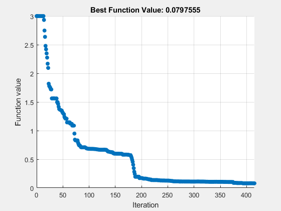
fprintf(formatstring,fval,output.funccount)
particleswarm reached the value 0.079755 using 24960 function evaluations.
Use More Particles
Frequently, using more particles obtains a more accurate solution.
rng default
options.SwarmSize = 200;
[x,fval,exitflag,output] = particleswarm(fun,nvars,lb,ub,options);
Optimization ended: relative change in the objective value over the last OPTIONS.MaxStallIterations iterations is less than OPTIONS.FunctionTolerance.
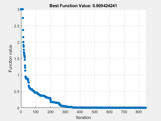
fprintf(formatstring,fval,output.funccount)
particleswarm reached the value 0.000424 using 169400 function evaluations.
Hybrid Function
particleswarm can search through several basins of attraction to arrive at a good local solution. Sometimes, though, it does not arrive at a sufficiently accurate local minimum. Try improving the final answer by specifying a hybrid function that runs after the particle swarm algorithm stops. Reset the number of particles to their original value, 60, to see the difference the hybrid function makes.
rng default
options.HybridFcn = @fmincon;
options.SwarmSize = 60;
[x,fval,exitflag,output] = particleswarm(fun,nvars,lb,ub,options);
Optimization ended: relative change in the objective value over the last OPTIONS.MaxStallIterations iterations is less than OPTIONS.FunctionTolerance.

fprintf(formatstring,fval,output.funccount)
particleswarm reached the value 0.000000 using 25191 function evaluations.
disp(output.hybridflag)
1
While the hybrid function improved the result, the plot function shows the same final value as before. This is because the plot function shows only the particle swarm algorithm iterations, and not the hybrid function calculations. The hybrid function caused the final function value to be very close to the true minimum value of 0. The output.hybridflag field shows that fmincon stops with exit flag 1, indicating that x is a true local minimum.