Gas Mileage Prediction Using ANFIS
This example shows how to predict fuel consumption for automobiles using data from previously recorded observations by training an ANFIS model.
Automobile miles per gallon (MPG) prediction is a typical nonlinear regression problem, in which several automobile features are used to predict fuel consumption in MPG. The training data for this example is available in the University of California, Irvine Machine Learning Repository and contains data collected from automobiles of various makes and models.
In this data set, the six input variables are number of cylinders, displacement, horsepower, weight, acceleration, and model year. The output variable to predict is the fuel consumption in MPG. In this example, you do not use the make and model information from the data set.
Partition Data
Obtain the data set from the original data file autoGas.dat using the loadGasData function.
[data,inputName] = loadGasData;
Partition the data set into a training set (odd-indexed samples) and a validation set (even-indexed samples).
trnData = data(1:2:end,:);
valData = data(2:2:end,:);
Select Inputs
Use the exhaustiveSearch function to perform an exhaustive search within the available inputs to select the set of inputs that most influence the fuel consumption. Use the first argument of exhaustiveSearch to specify the number of inputs per combination (1 for this example). exhaustiveSearch builds an ANFIS model for each combination, trains it for one epoch, and reports the performance achieved. First, use exhaustiveSearch to determine which variable by itself can best predict the output.
exhaustiveSearch(1,trnData,valData,inputName);
Train 6 ANFIS models, each with 1 inputs selected from 6 candidates...

Model 1: Cylinder, Error: trn = 4.6400, val = 4.7255
Model 2: Disp, Error: trn = 4.3106, val = 4.4316
Model 3: Power, Error: trn = 4.5399, val = 4.1713
Model 4: Weight, Error: trn = 4.2577, val = 4.0863
Model 5: Acceler, Error: trn = 6.9789, val = 6.9317
Model 6: Year, Error: trn = 6.2255, val = 6.1693
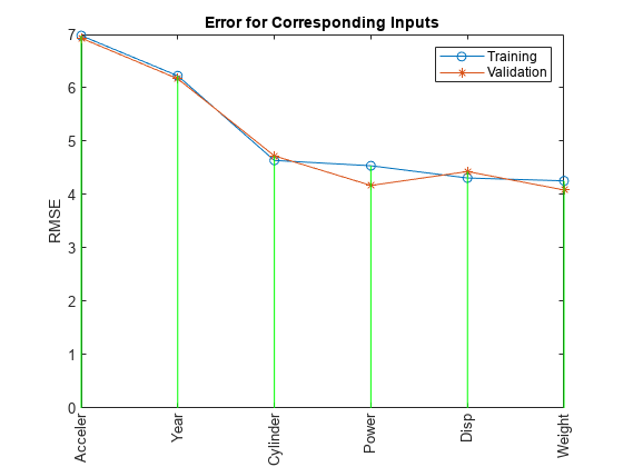
The graph indicates that the Weight variable has the lowest root mean squared error (RMSE). In other words, it can best predict MPG.
For Weight, the training and validation errors are comparable, indicating little overfitting. Therefore, you can likely use more than one input variable in your ANFIS model.
Although models using Weight and Disp individually have the lowest errors, a combination of these two variables does not necessarily produce the minimal training error. To identify which combination of two input variables results in the lowest error, use exhaustiveSearch to search every combination.
inputIndex = exhaustiveSearch(2,trnData,valData,inputName);
Train 15 ANFIS models, each with 2 inputs selected from 6 candidates...

ANFIS model 1: Cylinder Disp, Error: trn = 3.9320, val = 4.7920
ANFIS model 2: Cylinder Power, Error: trn = 3.7364, val = 4.8683
ANFIS model 3: Cylinder Weight, Error: trn = 3.8741, val = 4.6762
ANFIS model 4: Cylinder Acceler, Error: trn = 4.3287, val = 5.9625
ANFIS model 5: Cylinder Year, Error: trn = 3.7129, val = 4.5946
ANFIS model 6: Disp Power, Error: trn = 3.8087, val = 3.8594
ANFIS model 7: Disp Weight, Error: trn = 4.0271, val = 4.6352
ANFIS model 8: Disp Acceler, Error: trn = 4.0782, val = 4.4890
ANFIS model 9: Disp Year, Error: trn = 2.9565, val = 3.3905
ANFIS model 10: Power Weight, Error: trn = 3.9310, val = 4.2967
ANFIS model 11: Power Acceler, Error: trn = 4.2740, val = 3.8738
ANFIS model 12: Power Year, Error: trn = 3.3796, val = 3.3505
ANFIS model 13: Weight Acceler, Error: trn = 4.0875, val = 4.0094
ANFIS model 14: Weight Year, Error: trn = 2.7657, val = 2.9954
ANFIS model 15: Acceler Year, Error: trn = 5.6242, val = 5.6481
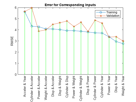
The results from exhaustiveSearch indicate that Weight and Year form the optimal combination of two input variables. However, the difference between the training and validation errors is larger than the difference for either variable alone, indicating that including more variables increases overfitting. Run exhaustiveSearch with combinations of three input variables to see whether these differences increase further with greater model complexity.
exhaustiveSearch(3,trnData,valData,inputName);
Train 20 ANFIS models, each with 3 inputs selected from 6 candidates...

ANFIS model 1: Cylinder Disp Power, Error: trn = 3.4446, val = 11.5329
ANFIS model 2: Cylinder Disp Weight, Error: trn = 3.6686, val = 4.8926
ANFIS model 3: Cylinder Disp Acceler, Error: trn = 3.6610, val = 5.2384
ANFIS model 4: Cylinder Disp Year, Error: trn = 2.5463, val = 4.9001
ANFIS model 5: Cylinder Power Weight, Error: trn = 3.4797, val = 9.3759
ANFIS model 6: Cylinder Power Acceler, Error: trn = 3.5432, val = 4.4804
ANFIS model 7: Cylinder Power Year, Error: trn = 2.6300, val = 3.6300
ANFIS model 8: Cylinder Weight Acceler, Error: trn = 3.5708, val = 4.8379
ANFIS model 9: Cylinder Weight Year, Error: trn = 2.4951, val = 4.0434
ANFIS model 10: Cylinder Acceler Year, Error: trn = 3.2698, val = 6.2616
ANFIS model 11: Disp Power Weight, Error: trn = 3.5879, val = 7.4951
ANFIS model 12: Disp Power Acceler, Error: trn = 3.5395, val = 3.9953
ANFIS model 13: Disp Power Year, Error: trn = 2.4607, val = 3.3563
ANFIS model 14: Disp Weight Acceler, Error: trn = 3.6075, val = 4.2323
ANFIS model 15: Disp Weight Year, Error: trn = 2.5617, val = 3.7858
ANFIS model 16: Disp Acceler Year, Error: trn = 2.4149, val = 3.2480
ANFIS model 17: Power Weight Acceler, Error: trn = 3.7884, val = 4.0471
ANFIS model 18: Power Weight Year, Error: trn = 2.4371, val = 3.2830
ANFIS model 19: Power Acceler Year, Error: trn = 2.7276, val = 3.2580
ANFIS model 20: Weight Acceler Year, Error: trn = 2.3603, val = 2.9152
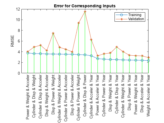
This plot shows the result of selecting three inputs. Here, the combination of Weight, Year, and Acceler produces the lowest training error. However, the training and validation errors are not substantially lower than that of the best two-input model, which indicates that the newly added variable Acceler does not improve the prediction much. As simpler models usually generalize better, use the two-input ANFIS for further exploration.
Extract the selected input variables from the original training and validation data sets.
newTrnData = trnData(:,[inputIndex, size(trnData,2)]);
newValData = valData(:,[inputIndex, size(valData,2)]);
Train ANFIS Model
The function exhaustiveSearch trains each ANFIS for only a single epoch to quickly find the right inputs. Now that the inputs are fixed, you can train the ANFIS model for more epochs.
Use the genfis function to generate an initial FIS from the training data, then use tunefis to fine-tune it.
opt = tunefisOptions(Method="anfis",Display="none");
opt.MethodOptions.EpochNumber = 100;
opt.MethodOptions.StepSizeDecreaseRate = 0.5;
opt.MethodOptions.StepSizeIncreaseRate = 1.5;
opt.MethodOptions.ValidationData = newValData;

inFIS = genfis(newTrnData(:,1:end-1),newTrnData(:,end));
[in,out] = getTunableSettings(inFIS);

[trnOutFIS,summary] = tunefis(inFIS,[in;out],newTrnData(:,1:end-1),newTrnData(:,end),opt);
trnError = summary.tuningOutputs.trainError;
valError = summary.tuningOutputs.chkError;
valOutFIS = summary.tuningOutputs.chkFIS;
tunefis returns the training and validation errors in its summary output argument. Plot the training and validation errors over the course of the training process.
[minValError,b] = min(valError);
plot(1:100,trnError,"g-",1:100,valError,"r-",b,minValError,"ko")
title("Training (green) and validation (red) error curve")
xlabel("Epoch number")
ylabel("RMSE")
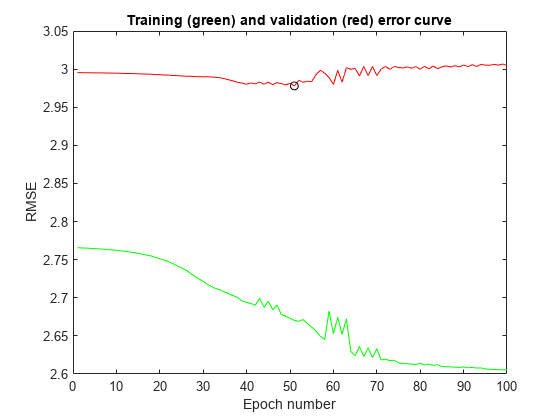
This plot shows the error curves for 100 epochs of ANFIS training. The green curve gives the training errors and the red curve gives the validation errors. The minimal validation error occurs at about epoch 45, which is indicated by a circle. Notice that the validation error curve goes up after 50 epochs, indicating that further training overfits the data and produces increasingly worse generalization.
Analyze ANFIS Model
First, compare the performance of the ANFIS model with that of a linear model using their respective validation RMSE values.
You can compare the ANFIS prediction against a linear regression model by comparing their respective RMSE values against the validation data.
% Perform linear regression.
N = size(trnData,1);
A = [trnData(:,1:6) ones(N,1)];
B = trnData(:,7);
coef = A\B; % Solve for regression parameters from training data.

Nc = size(valData,1);
A_ck = [valData(:,1:6) ones(Nc,1)];
B_ck = valData(:,7);
lrRMSE = norm(A_ck*coef-B_ck)/sqrt(Nc);

fprintf("RMSE against validation data:\n")
RMSE against validation data:
fprintf("ANFIS: %1.3f\tLinear Regression: %1.3f\n",minValError,lrRMSE)ANFIS: 2.976 Linear Regression: 3.444
The ANFIS model has a lower validation RMSE and therefore outperforms the linear regression model.
The variable valOutFIS is a snapshot of the ANFIS model at the minimal validation error during the training process. Plot an output surface of the model.
valOutFIS.Inputs(1).Name = "Weight";
valOutFIS.Inputs(2).Name = "Year";
valOutFIS.Outputs(1).Name = "MPG";

gensurf(valOutFIS)
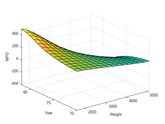
The output surface is nonlinear and monotonic and illustrates how the ANFIS model responds to varying values of Weight and Year.
The surface indicates that, for vehicles manufactured in or after 1978, heavier automobiles are more efficient. Plot the data distribution to see any potential gaps in the input data that might cause this counterintuitive result.
plot(newTrnData(:,1),newTrnData(:,2),"bo", ...
     newValData(:,1),newValData(:,2),"rx")
xlabel("Weight")
ylabel("Year")
title("Training (o) and Validation (x) Data")
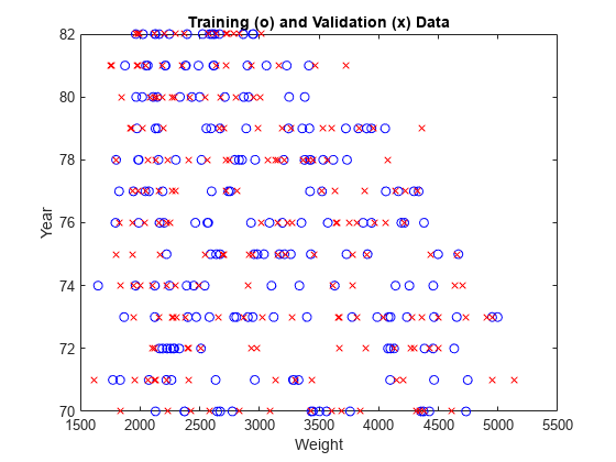
The lack of training data for heavier vehicles manufactured in later years causes the anomalous results. Because data distribution strongly affects prediction accuracy, take the data distribution into account when you interpret the ANFIS model.
See Also
tunefis | tunefisOptions | genfis | evalfis