Implement HDL-Optimized Real QRD-RLS Adaptive Filtering

R2026b

This example shows how to implement real QR decomposition-based recursive least squares (QRD-RLS) adaptive filtering for system identification. The example includes a MATLAB® fixed-point implementation and a Simulink® model implementation optimized for HDL code generation.

The QRD-RLS algorithm is a variation of the RLS algorithm that uses QR-decomposition to preserve numerical stability in finite-precision implementations. You can use the QRD-RLS algorithm to estimate a linear model from measured input-output data that minimizes a specific cost function.

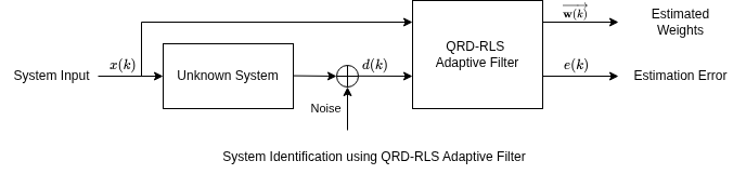
In this example, the unknown system is a tapped-delay line FIR filter of order $N-1$ with $N\times 1$ weight coefficient vector $\overrightarrow{\underset{}{w}}$. Both the coefficients and the input signal are real numbers. For each time step $k$, a scalar input signal $x\left(k\right)$ is fed into the unknown system, and the resulting output is measured as a desired output signal $d\left(k\right)$. The adaptive filter takes $x\left(k\right)$ and $d\left(k\right)$ as inputs and estimates $\overrightarrow{\underset{}{w}}$ each time step as $\overrightarrow{\underset{}{\underset{}{\overset{ˆ}{w}}\left(k\right)}}$. For this following weighted least-squares cost function with exponential forgetting factor $\alpha$ and Tikhonov regularization parameter $\lambda$:

$J\left(\overrightarrow{\underset{}{w}},k\right)={\lambda }^2{\alpha }^k||\overrightarrow{\underset{}{w}}|{|}^2+\sum _{i=0}^k{\alpha }^{k-i}{\left[d\left(i\right)-\overrightarrow{\underset{}{w^H}}\overrightarrow{\underset{}{x\left(k\right)}}\right]}^2$, where $\overrightarrow{\underset{}{x\left(k\right)}}=\left[\begin{array}{c}x\left(k\right)\\ x\left(k-1\right)\\ ⋮\\ x\left(k-N\right)\end{array}\right]$ is the last $N$ tapped samples of $x\left(k\right)$,

the estimations $\overrightarrow{\underset{}{\underset{}{\overset{ˆ}{w}}\left(k\right)}}=\underset{\overrightarrow{\underset{}{w}}}{argmin}J\left(\overrightarrow{\underset{}{w}},k\right)$ minimize this cost function for each time step.

The a-posteriori estimation error $e\left(k\right)$ is also computed by the adaptive filter. This error is defined as $e\left(k\right)=d\left(k\right)-{\overrightarrow{\underset{}{w\left(k\right)}}}^H\overrightarrow{\underset{}{x\left(k\right)}}$.

Define Unknown System and Generate Input Data

Design the unknown system as an $N-1$ order FIR filter with a normalized cutoff frequency of 0.25 radians.

N = 11;
w = designLowpassFIR(FilterOrder=N-1, CutoffFrequency=0.25)

w = 1×11

   -0.0039    0.0000    0.0321    0.1167    0.2207    0.2687    0.2207    0.1167    0.0321    0.0000   -0.0039

system_unknown = dsp.FIRFilter('Numerator',w);

Generate $K$ samples of random Gaussian data, $x\left(k\right)$. Generate a noisy measurement of the output of the unknown system, $d\left(k\right)$.

K = 150;
x = randn(K, 1);
n = 0.01*randn(K,1);
d = system_unknown(x) + n;

Apply Floating Point QRD-RLS Adaptive Filter

To establish a floating-point reference for the fixed-point implementation, use the dsp.RLSFilter (DSP System Toolbox) System object™. To specify the QRD-RLS algorithm, set the Method parameter to 'qr-decomposition rls'. Use the floating-point results to validate fixed-point estimations of $\overrightarrow{\underset{}{\underset{}{\overset{ˆ}{w}}\left(k\right)}}$ and the estimation error profile $e\left(k\right)$.

Define forgetting factor $\alpha$ and Tikhonov regularization parameter $\lambda$. The forgetting factor controls the exponential rate at which older input data is de-emphasized. The Tikhonov regularization parameter $\lambda$ is used to initially bias the weight estimation to improve numerical stability. This bias can also reduce mean squared error compared to pure least-squares estimates.

forgettingFactor = 0.98;
regularizationParameter = sqrt(1e-3);
qrd_rls = dsp.RLSFilter(N,"ForgettingFactor",forgettingFactor,'InitialSquareRootCovariance',regularizationParameter,'Method','qr-decomposition rls');
[~,e_reference] = qrd_rls(x,d);
w_reference = qrd_rls.Coefficients

w_reference = 1×11

   -0.0033    0.0011    0.0323    0.1163    0.2214    0.2695    0.2219    0.1180    0.0327   -0.0003   -0.0021

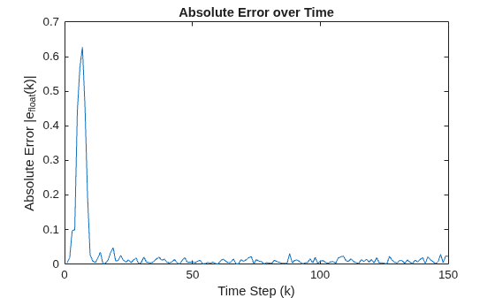
Plot the absolute prediction error $|e\left(k\right)|$. The error converges toward zero over time in the presence measurement noise. The dsp.RLSFilter object calculates a-priori error that is defined as $e\left(k\right)=d\left(k\right)-{\overrightarrow{\underset{}{w\left(k\right)}}}^H\overrightarrow{\underset{}{x\left(k-1\right)}}$, so it displays an expected initial error spike before settling as the filter adapts.

plot(abs(e_reference))
title("Absolute Error over Time")
xlabel("Time Step (k)")
ylabel("Absolute Error |e_{float}(k)|")

Implement Fixed-Point QRD-RLS MATLAB Algorithm

Implement the QRD-RLS algorithm with fixed-point data. Use the floating-point results as an accuracy reference.

Specify Input Data Type

Use the DT drop-down list to select a double-precision or a fixed-point input data type. When you select fixed, the example uses fixed-point data types chosen experimentally to avoid overflow in the Simulink model.

DT = 'fixed';
if strcmp(DT,'fixed')
    wordLength = 32;
    fractionalLength = 23;
    OutputType = fixdt(1,32,28);
    inputType = numerictype(1,wordLength,fractionalLength);
else
    inputType = 'double';
    OutputType = 'double';
end

inputPrototype = fixed.numerictypeToPrototype(inputType);
outputPrototype = fixed.numerictypeToPrototype(OutputType);
x = cast(x,"like",inputPrototype);
d = cast(d,"like",inputPrototype);

The MATLAB implementation expresses the algorithm as a sequence of operations that translate into a Simulink model. Each time step, the algorithm maintains and updates an upper-triangular system using Givens rotations. The algorithm solves the system each time step to estimate $\overrightarrow{\underset{}{\underset{}{\overset{ˆ}{w}}\left(k\right)}}$.

The algorithm maintains upper-triangular $N\times N$ matrix $R\left(k\right)$ and $N\times 1$ column vector $\overrightarrow{\underset{}{d_{q2}\left(k\right)}}$ as internal states. The algorithm stores them in the matrix structure,

$\left[\begin{array}{ccc}R\left(k\right)& \overrightarrow{\underset{}{d_{q2}\left(k\right)}}& \left[\begin{array}{c}0\\ ⋮\\ 0\end{array}\right]\end{array}\right]$,

and initializes them as,

$R\left(-1\right)={\lambda I}_N$ and $\overrightarrow{\underset{}{d_{q2}\left(-1\right)}}=\overrightarrow{\underset{}{0}}$,

for Tikhonov regularization parameter $\lambda$.

Each time step, the algorithm collects $\overrightarrow{\underset{}{x\left(k\right)}}$ and $d\left(k\right)$ to form the $1\times \left(N+2\right)$ update vector $\left[\begin{array}{ccc}\overrightarrow{\underset{}{x^T\left(k\right)}}& d\left(k\right)& 1\end{array}\right]$. Appending this vector to the bottom of the internal state matrix disturbs the upper-triangular structure. $R\left(k\right)$ and $\overrightarrow{\underset{}{d_{q2}\left(k\right)}}$ are scaled by the square root of the forgetting factor, $\alpha$, and Givens rotations are performed to zero out the bottom-left entries of the augmented matrix, which restores the triangular structure. This process updates the values of $R\left(k\right)$ and $\overrightarrow{\underset{}{d_{q2}\left(k\right)}}$ and produces two scalar values, $e_{q1}\left(k\right)$ and $\gamma \left(k\right)$. The update operation is represented by this relation:

$\left[\begin{array}{ccc}{\alpha }^{\frac{1}{2}}R\left(k-1\right)& {\alpha }^{\frac{1}{2}}\overrightarrow{\underset{}{d_{q2}\left(k-1\right)}}& \left[\begin{array}{c}0\\ ⋮\\ 0\end{array}\right]\\ \overrightarrow{\underset{}{x^T\left(k\right)}}& d\left(k\right)& 1\end{array}\right]\underset{Q-lessQRUpdate}{⟹}\left[\begin{array}{ccc}R\left(k\right)& \overrightarrow{\underset{}{d_{q2}\left(k\right)}}& \left[\begin{array}{c}*\\ ⋮\\ *\end{array}\right]\\ \left[\begin{array}{ccc}0& \cdots & 0\end{array}\right]& e_{q1}\left(k\right)& \gamma \left(k\right)\end{array}\right]$,

where $*$ denotes an unused value.

The system of equations represented by $R\left(k\right)$ and $\overrightarrow{\underset{}{d_{q2}\left(k\right)}}$ is then solved using backward substitution to estimate $\overrightarrow{\underset{}{\underset{}{\overset{ˆ}{w}}\left(k\right)}}$,

$\overrightarrow{\underset{}{\underset{}{\overset{ˆ}{w}}\left(k\right)}}=R^{-1}\left(k\right)\overrightarrow{\underset{}{d_{q2}\left(k\right)}}$.

The scalar factors $e_{q1}\left(k\right)$ and $\gamma \left(k\right)$ are used to calculate the a-posteriori estimation error $e\left(k\right)$ through scalar multiplication,

$e\left(k\right)=e_{q1}\left(k\right)\gamma \left(k\right)$.

In the realQRDRLS function, the qlessQRUpdate function maps directly to the update equation.

updateVector = [x_k,d(1),cast(1,'like',x)];

[R_augmented(:),updateVector(:)] = qlessQRUpdate([R,dq2,zeros(N,1)],updateVector,sqrtForgettingFactor);

type("realQRDRLS.m");

function [e,w,ROut] = realQRDRLS(x,d,N,OutputType,forgettingFactor,regularizationParameter)
%realQRDRLS This function perform the QRD-RLS algorithm for real number. If
%input is fixed-point type, it provides bit-exact results with the example
%model
%
%   [e, w, ROut] = realQRDRLS(x, d, OutputType, forgettingFactor,
%   regularizationParameter) x is the signal to be filtered by the RLS
%   filter, d is the reference signal, OutputType is the output type of e
%   and w, forgetting factor is RLS forgetting factor, regularization
%   parameter is the initial square root covariance. 
%   
%   e is the difference between the output signal y and the desired signal
%   d, w is the estimated filter coefficients, ROut is the covariance
%   matrix and dq2, [R dq2], ROut has same datatype with x.
%
%   Copyright 2026 The MathWorks, Inc.

%#codegen
coder.const(N);
coder.const(forgettingFactor);

% The HDL Optimized block directly apply the square root of the forgetting
% factor to the internal covariance matrix while dsp.RLSFilter compute the
% square root internally. Such that the square root of the forgetting
% factor is pre-computed as a constant.
sqrtForgettingFactor = coder.const(sqrt(forgettingFactor));

coder.const(regularizationParameter);
outputPrototype = coder.const(fixed.numerictypeToPrototype(OutputType));
K = coder.const(numel(x));

x_k = zeros(1,N,"like",x);
w = zeros(1,N,"like",outputPrototype);
e = zeros(K,1,"like",outputPrototype);


eq1 = zeros(1,1,"like",x);
eq1 = setfimath(eq1,fixed.fimathLike(eq1));
gamma = zeros(1,1,"like",x);
dq2 = zeros(N,1,"like",x);
R = cast(regularizationParameter*eye(N,N),'like',x);
ROut = [R dq2];

R_augmented = zeros(N,N+2,'like',x);
updateVector = [x_k, d(1), cast(1,'like',x)];

for k=1:K
    x_k(:) = [x(k), x_k(1:end-1)];
    updateVector(:) = [x_k, d(k), 1];
    % Each time step, use one pair of input and reference output to update
    % R matrix
    [R_augmented(:), updateVector(:)] = qlessQRUpdate([R, dq2, zeros(N,1)], updateVector, sqrtForgettingFactor);
    R(:) = R_augmented(1:N,1:N);
    dq2(:) = R_augmented(1:N, N+1);
    gamma(:) = updateVector(end,end);
    eq1(:) = updateVector(end, end-1);
    e(k) = eq1 * gamma;
end

w(:) = fixed.backwardSubstitute(R, dq2, OutputType);
ROut(:) = [R dq2];

end

[e,w] = realQRDRLS(x,d,N,outputPrototype,forgettingFactor,regularizationParameter);

If you set data type DT to fixed, the realQRDRLS function can run slowly in MATLAB interpreted mode for large fixed-point data sets. Use the fiaccel function to accelerate the fixed-point simulation.

fiaccel realQRDRLS -args {x, d, coder.Constant(N), coder.Constant(outputPrototype), coder.Constant(forgettingFactor), coder.Constant(regularizationParameter)}
[e,w,ROut] = realQRDRLS_mex(x,d,N,outputPrototype,forgettingFactor,regularizationParameter);

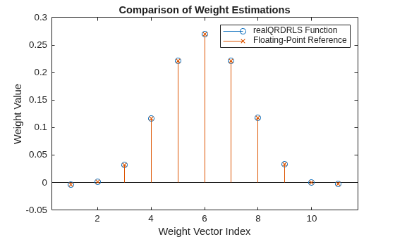
Compare the $\overrightarrow{\underset{}{\underset{}{\overset{ˆ}{w}}\left(k\right)}}$ estimate of the fixed-point implementation to the floating-point reference at time step $k=K$.

stem(double(w));
hold on
stem(w_reference,'-x');
hold off
title("Comparison of Weight Estimations")
legend('realQRDRLS Function','Floating-Point Reference');
xlabel('Weight Vector Index'); 
ylabel('Weight Value');

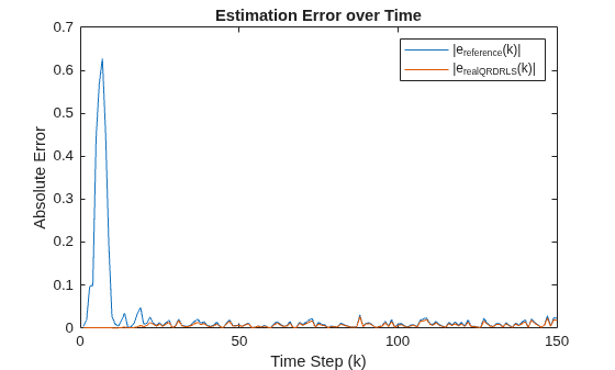
Plot the estimation error profiles between the fixed-point implementation and the dsp.RLSFilter implementation. The fixed-point implementation reports zero a-posteriori error for time steps $k<N$, whereas the dsp.RLSFilter function calculates the a-priori error. The two error profiles converge at later time steps.

plot(1:K, [abs(e_reference), abs(double(e))])
title("Estimation Error over Time")
xlabel("Time Step (k)")
ylabel("Absolute Error")
legend("|e_{reference}(k)|", "|e_{realQRDRLS}(k)|")

Implement HDL-Optimized QRD-RLS Algorithm in Simulink

The QRD_RLS model implements the same fixed-point QRD-RLS algorithm as the MATLAB function realQRDRLS. The model adds HDL-optimized components for system simulation and code generation.

Open the QRD_RLS model.

model = 'QRD_RLS';
open_system(model);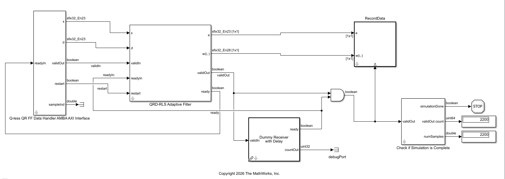

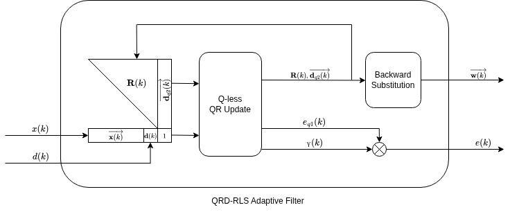
The diagram below shows the datapath of the HDL-optimized QRD-RLS Adaptive Filter block in the model. Each step, the input signal $x$, desired output signal $d$, and a constant number $1$ form the update vector. The CORDIC-based Q-less QR Update kernel processes this vector to update the covariance matrix $R$. The a-posteriori estimation error $e$ is then computed by scalar multiplication, and the weights estimation is computed by backward substitution.

Testbench setup and I/O interface

The Data Handler subsystem reads data signals $x\left(k\right)$ and $d\left(k\right)$ from the model workspace and feeds them sample-by-sample into the QRD-RLS Adaptive Filter block using the AMBA-AXI interface. The validIn signal indicates when new input data is available. The ready signal indicates when the subsystem can accept data. Data transfer occurs only when both the validIn and ready signals are high. You can set a delay between the availability of data samples in the Data Handler to emulate the processing time of the upstream block.

upstreamDelay = 0;

The Dummy Receiver with Delay subsystem models downstream data processing time. The readyIn input of the QRD-RLS Adaptive Filter block indicates when the downstream component is ready to accept the output data. You can set downstream delay to emulate backpressure in the system.

downstreamDelay = 0;

Use the helper function setModelWorkspace to add all the parameters defined above to the model workspace.

fixed.example.setModelWorkspace(model,'A',x,'D',d,'N',N,...
    'regularizationParameter',regularizationParameter,'forgettingFactor',sqrt(forgettingFactor),'numSamples', K,...
    'upstreamDelay',0,'restartDelay',0,'downstreamDelay',0,'OutputType',OutputType);

Simulate the model.

simout = sim(model);
data_out = simout.data_Out;
e_out = simout.e_Out;

The QRD-RLS Adaptive Filter block outputs individual elements of $\overrightarrow{\underset{}{\underset{}{\overset{ˆ}{w}}\left(k\right)}}$ and the current $e\left(k\right)$ scalar value each handshake, which the Record Data subsystem collects as two $K*N$ length vectors.

Extract the $K$ $\overrightarrow{\underset{}{\underset{}{\overset{ˆ}{w}}\left(k\right)}}$ vectors and corresponding $e\left(k\right)$ scalar values. If the output contains R or w, compare the output of the Simulink model to the floating-point reference at time step $k=K$.

e_model = zeros(K,1,"like",fixed.numerictypeToPrototype(OutputType));
w_k_model = zeros(K,N,'like',outputPrototype);
for k = 1:K
    w_k_model(k,:) = data_out((1:N) + (N*(k-1)));
    e_model(k) = e_out(N*(k-1) + 1);
end
w_model = w_k_model(K,:);

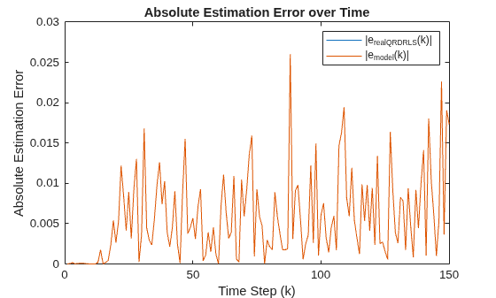
Plot a comparison of the estimation error profiles between the QRD_RLS Simulink model implementation and the realQRDRLS function implementation in MATLAB.

plot(1:K,[abs(e),abs(e_model)])
title("Absolute Estimation Error over Time")
xlabel("Time Step (k)")
ylabel("Absolute Estimation Error")
legend("|e_{realQRDRLS}(k)|","|e_{model}(k)|")

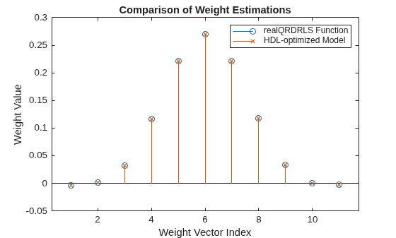
Plot a comparison of the weights estimated by the Simulink model and the output of the realQRDRLS function.

stem(w);
hold on
stem(w_model,'-x');
hold off
title("Comparison of Weight Estimations")
legend('realQRDRLS Function','HDL-optimized Model');
xlabel('Weight Vector Index'); 
ylabel('Weight Value');

For fixed-point input data, confirm that the MATLAB implementation realQRDRLS and the Simulink HDL-optimized QRD-RLS Adaptive Filter block implementation produce bit-exact results.

if strcmp(DT,'fixed')
    eBitExact = ispropequal(e,e_model)
    wBitExact = ispropequal(w,w_model)
end

eBitExact = logical
   1

wBitExact = logical
   1

Hardware Performance

The latency of the QRD-RLS Adaptive Filter block is defined as the number of clock cycles between a valid input to the corresponding valid output. The latency scales with the input word length and the number of filter taps as $L\times N+N^2$, where $L$ is the input word length and $N$ is the number of taps.

The input/output interval is defined as the number of clock cycles between adjacent inputs or outputs. This interval scales with the input word length and the number of filter taps as $L\times N$.

To measure the latency and the input/output interval in Simulink, log the input and output handshaking signals and view them in the Logic Analyzer. This figure shows timing for a 32-bit data type with 11 taps. The first valid input is located at step 0, and the first valid output is located at step 595, giving a latency of 595. The second output occurs at step 1025 cycles, giving an input/output interval of 430 cycles.

To extract the latency information programmatically, use the extractLatency helper function.

[measuredIOInterval, measuredLatency] = extractLatency(simout, N, K);

Synthesis Results for Various Output Combinations

For applications that do not require weight estimation, you can remove the backward substitution to save hardware resources and reduce computation time. The QRD-RLS Adaptive Filter block in this example supports three output combinations that you can configure using the block parameter outputOption. This table describes supported configurations and use cases.

Output Combination	Hardware Configuration	Notes
'e'	No backward substitution	Suitable for applications that don't need weight estimation.
'e and R'	No backward substitution	Output e and internal matrix [R dq2]. This configuration is suitable for applications that require the backward substitution to be processed in another place, such as the processor on an SoC.
'e and w'	With backward substitution	Estimate weights in hardware.

The QRD-RLS Adaptive Filter block in this example supports HDL code generation using the Simulink® HDL Workflow Advisor. For examples, see HDL Code Generation and FPGA Synthesis from Simulink Model (HDL Coder) and Implement Digital Downconverter for FPGA (DSP HDL Toolbox).

This example data was generated by synthesizing the block on an AMD® Zynq®-7 ZC706 evaluation board (-2 speed grade) using Vivado® v2025.1.1

These tables show the synthesis resource utilization results and timing summary with different output combinations.

Output combination 'e and w'

Resource	Usage	Available	Utilization (%)
Slice LUTs	23022	218600	10.53
Slice Registers	7959	437200	1.82
DSPs	60	900	6.67
Block RAM Tile	0	545	0.00
URAM	0	0	0.00

Timing Metric	Value
Requirement	5 ns (200 MHz)
Data Path Delay	3.051 ns
Slack	0.892 ns
Clock Frequency	243.43 MHz

Output combination 'e and R'

Resource	Usage	Available	Utilization (%)
Slice LUTs	19764	218600	9.04
Slice Registers	5149	437200	1.18
DSPs	52	900	5.78
Block RAM Tile	0	545	0.00
URAM	0	0	0.00

Timing Metric	Value
Requirement	5 ns (200 MHz)
Data Path Delay	3.051 ns
Slack	0.892 ns
Clock Frequency	243.43 MHz

Output combination 'e'

Resource	Usage	Available	Utilization (%)
Slice LUTs	19153	218600	8.76
Slice Registers	4374	437200	1.00
DSPs	52	900	5.78
Block RAM Tile	0	545	0.00
URAM	0	0	0.00

Timing Metric	Value
Requirement	5 ns (200 MHz)
Data Path Delay	3.051 ns
Slack	0.892 ns
Clock Frequency	243.43 MHz

References

[1] Apolinário Jr, José Antonio. QRD-RLS Adaptive Filtering. Springer, 2009.

[2] Bertheussen, Andreas. "Adaptive Beamforming Using the Recursive Least Squares Algorithm on an FPGA." Master's thesis, Norwegian University of Science and Technology, 2015.

See Also

fixed.qlessQR

Topics

Overview of Adaptive Filters and Applications (DSP System Toolbox)