Compute Quantization Error

This example shows how to compute and compare the statistics of the signal quantization error when using various rounding methods. Quantization occurs when a data type cannot represent a value exactly. In these cases, the value must be rounded to the nearest value that can be represented by the data type.

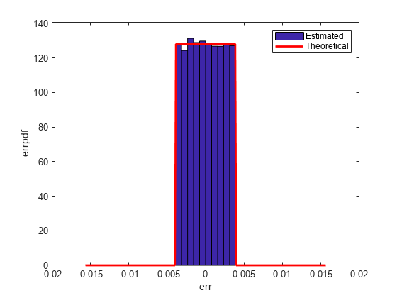
First, a random signal is created that spans the range of the quantizer object. Next, the signal is quantized, respectively, with rounding methods 'fix', 'floor', 'ceil', 'nearest', and 'convergent', and the statistics of the signal are estimated.

The theoretical probability density function of the quantization error is computed with the errpdf function, the theoretical mean of the quantization error is computed with the errmean function, and the theoretical variance of the quantization error is computed with the errvar function.

Create Uniformly Distributed Random Signal

Create a uniformly distributed random signal that spans the domain -1 to 1 of the fixed-point quantizer object q.

q = quantizer([8 7]);
r = realmax(q);
u = r*(2*rand(50000,1) - 1);
xi = linspace(-2*eps(q),2*eps(q),256);

Fix: Round Towards Zero

With 'fix' rounding, the probability density function is twice as wide as the others. For this reason, the variance is four times that of the others.

q = quantizer('fix',[8 7]);
err = quantize(q,u) - u;    
f_t = errpdf(q,xi);
mu_t = errmean(q);
v_t  = errvar(q);

qerrordemoplot(q,f_t,xi,mu_t,v_t,err)

Estimated   error variance (dB) = -46.8586
Theoretical error variance (dB) = -46.9154
Estimated   mean = 7.788e-06
Theoretical mean = 0

The theoretical variance is eps(q)^2/3 and the theoretical mean is 0.

Floor: Round Towards Negative Infinity

'floor' rounding is often called truncation when used with integers and fixed-point numbers that are represented using two's complement notation. It is the most common rounding mode of DSP processors because it requires no hardware to implement. 'floor' does not produce quantized values that are as close to the true values as 'round' will, but it has the same variance. Using 'floor', small signals that vary in sign will be detected, whereas in 'round' they will be lost.

q = quantizer('floor',[8 7]);
err = quantize(q,u) - u;    
f_t = errpdf(q,xi);
mu_t = errmean(q);
v_t = errvar(q);

qerrordemoplot(q,f_t,xi,mu_t,v_t,err)

Estimated   error variance (dB) = -52.9148
Theoretical error variance (dB) = -52.936
Estimated   mean = -0.0038956
Theoretical mean = -0.0039062

The theoretical variance is eps(q)^2/12 and the theoretical mean is -eps(q)/2.

Ceil: Round Towards Positive Infinity

q = quantizer('ceil',[8 7]);
err = quantize(q,u) - u;    
f_t = errpdf(q,xi);
mu_t = errmean(q);
v_t  = errvar(q);

qerrordemoplot(q,f_t,xi,mu_t,v_t,err)

Estimated   error variance (dB) = -52.9148
Theoretical error variance (dB) = -52.936
Estimated   mean = 0.0039169
Theoretical mean = 0.0039062

The theoretical variance is eps(q)^2/12 and the theoretical mean is eps(q)/2.

Round: Round to Nearest; In a Tie Round to Largest Magnitude

'round' is more accurate than 'floor', but all values smaller than eps(q) get rounded to zero and are lost.

q = quantizer('nearest',[8 7]);
err = quantize(q,u) - u;    
f_t = errpdf(q,xi);
mu_t = errmean(q);
v_t  = errvar(q);

qerrordemoplot(q,f_t,xi,mu_t,v_t,err)

Estimated   error variance (dB) = -52.9579
Theoretical error variance (dB) = -52.936
Estimated   mean = -2.212e-06
Theoretical mean = 0

The theoretical variance is eps(q)^2/12 and the theoretical mean is 0.

Convergent: Round to Nearest; In a Tie Round to Even

'convergent' rounding eliminates the bias introduced by ordinary 'round' caused by always rounding the tie in the same direction.

q = quantizer('convergent',[8 7]);
err = quantize(q,u) - u;    
f_t = errpdf(q,xi);
mu_t = errmean(q);
v_t  = errvar(q);

qerrordemoplot(q,f_t,xi,mu_t,v_t,err)

Estimated   error variance (dB) = -52.9579
Theoretical error variance (dB) = -52.936
Estimated   mean = -2.212e-06
Theoretical mean = 0

The theoretical variance is eps(q)^2/12 and the theoretical mean is 0.

Compare Nearest and Convergent Rounding

The error probability density function for convergent rounding is difficult to distinguish from that of round-to-nearest by looking at the plot.

The error probability density function of convergent is

f(err) = 1/eps(q),  for -eps(q)/2 <= err <= eps(q)/2, and 0 otherwise

while the error probability density function of round is

f(err) = 1/eps(q),  for -eps(q)/2 <  err <= eps(q)/2, and 0 otherwise

The error probability density function of convergent is symmetric, while round is slightly biased towards the positive.

The only difference is the direction of rounding in a tie.

x = (-3.5:3.5)';
[x convergent(x) nearest(x)]

ans = 8×3

   -3.5000   -4.0000   -3.0000
   -2.5000   -2.0000   -2.0000
   -1.5000   -2.0000   -1.0000
   -0.5000         0         0
    0.5000         0    1.0000
    1.5000    2.0000    2.0000
    2.5000    2.0000    3.0000
    3.5000    4.0000    4.0000