Perform GARCH Model Residual Diagnostics Using Econometric Modeler App

This example shows how to evaluate GARCH model assumptions by performing residual diagnostics using the Econometric Modeler app. The data set, stored in CAPMuniverse.mat available with the Financial Toolbox™ documentation, contains market data for daily returns of stocks and cash (money market) from the period January 1, 2000 to November 7, 2005. Consider modeling the market index returns (MARKET).

Import Data into Econometric Modeler

Download the CAPMuniverse.mat MAT-file into your current folder, and then load it into the workspace.

fldr = pwd;
openExample("CAPMuniverse.mat",workDir=fldr);
load(fullfile(fldr,"CAPMuniverse.mat"))

To change the folder to which to download the data set, set fldr to its absolute path.

The series are in the timetable AssetsTimeTable. The first column of data (AAPL) is the daily return of a technology stock. The last column is the daily return for cash (the daily money market rate, CASH).

At the command line, open the Econometric Modeler app.

econometricModeler

Alternatively, open the app from the apps gallery (see Econometric Modeler).

Import AssetsTimeTable into the app:

1. On the Modeler tab, in the Import section, click .

2. In the Import Data dialog box, select the check box for the AssetsTimeTable variable.

3. Click Import.

The market index variables, including MARKET, appear in the Time Series pane, and a time series plot containing all the series appears in the Plot(APPL) figure window.

Plot the Series

Plot the market index series by double-clicking the MARKET time series in the Time Series pane.

The series appears to fluctuate around y = 0 and exhibits volatility clustering. Consider a GARCH(1,1) model without a mean offset for the series.

Specify and Estimate GARCH Model

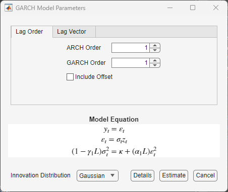
Specify a GARCH(1,1) model without a mean offset.

1. In the Time Series pane, select MARKET.

2. On the Modeler tab, in the Models section, click the arrow to display the models gallery.

3. In the models gallery, in the GARCH Models section, click GARCH.

4. In the GARCH Model Parameters dialog box, on the Lag Order tab, , clear the Include Offset check box, then click Estimate.

   

The model variable GARCH_MARKET appears in the Models pane, its value appears in the Preview pane, and its estimation summary appears in the Fit(GARCH_MARKET) document.

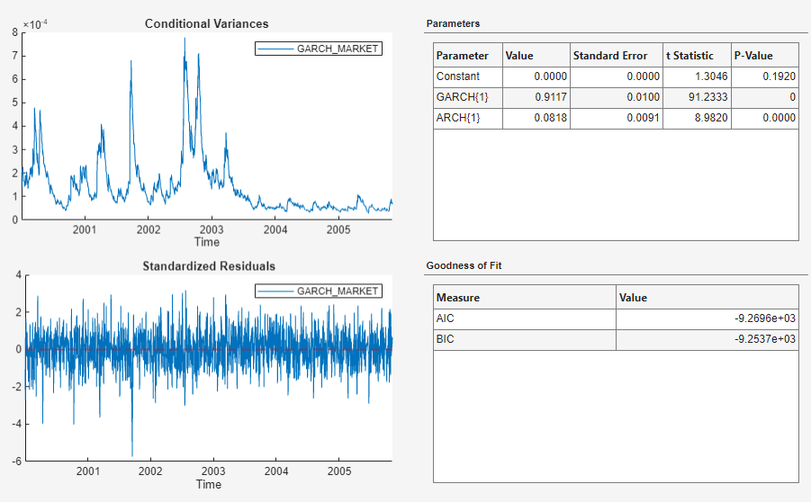
The p values of the coefficient estimates are close to zero, which indicates that the estimates are significant. The inferred conditional variances show high volatility through 2003, then small volatility through 2005. The standardized residuals appear to fluctuate around y = 0, and there are several large (in magnitude) residuals.

Check Goodness of Fit

Assess whether the standardized residuals are normally distributed and uncorrelated. Then, assess whether the residual series has lingering conditional heteroscedasticity.

Assess whether the standardized residuals are normally distributed by plotting their histogram and a quantile-quantile plot:

1. In the Models pane, select GARCH_MARKET.

2. On the Modeler tab, in the Diagnostics section, click Model Fit Diagnostics > Residual Histogram.

3. In the Diagnostics section, click Model Fit Diagnostics > Residual Q-Q Plot.

The histogram and quantile-quantile plot appear in the Hist(GARCH_MARKET) and QQ(GARCH_MARKET) figure windows, respectively.

Assess whether the standardized residuals are autocorrelated by plotting their autocorrelation function (ACF).

1. In the Models pane, select GARCH_MARKET.

2. On the Modeler tab, in the Diagnostics section, click Model Fit Diagnostics > Residual Autocorrelation.

The ACF plot appears in the ACF(GARCH_MARKET) figure window.

Assess whether the residual series has lingering conditional heteroscedasticity by plotting the ACF of the squared standardized residuals:

1. In the Models pane, select GARCH_MARKET.

2. Click the Modeler tab. Then, in the Diagnostics section, click Model Fit Diagnostics > Squared Residual Autocorrelation.

The ACF of the squared standardized residuals appears in the ACF(GARCH_MARKET)_2 figure window.

Arrange the histogram, quantile-quantile plot, ACF, and the ACF of the squared standardized residual series so that they occupy the four quadrants of the right pane. On the Documents pane, click the Document actions button , select Tile All, place the pointer in the (2,2) position of the matrix of squares.

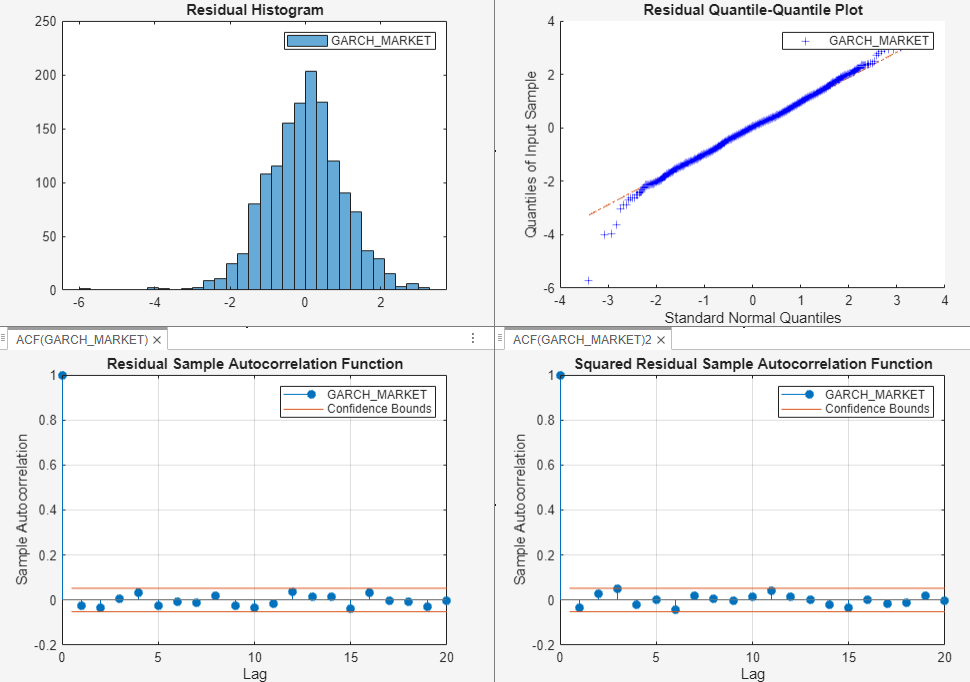
Although the results show a few large standardized residuals, they appear to be approximately normally distributed. The ACF plots of the standardized and squared standardized residuals do not contain any significant autocorrelations. Therefore, it is reasonable to conclude that the standardized residuals are uncorrelated and homoscedastic.