Nonseasonal Differencing
This example shows how to take a nonseasonal difference of a time series. The time series is quarterly U.S. GDP measured from 1947 to 2005.
Load the GDP data set included with the toolbox.
load Data_GDP
Y = Data;
N = length(Y);

figure
plot(Y)
xlim([0,N])
title('U.S. GDP')
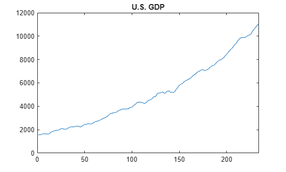
The time series has a clear upward trend.
Take a first difference of the series to remove the trend,
First create a differencing lag operator polynomial object, and then use it to filter the observed series.
D1 = LagOp({1,-1},'Lags',[0,1]);
dY = filter(D1,Y);

figure
plot(2:N,dY)
xlim([0,N])
title('First Differenced GDP Series')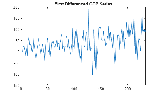
The series still has some remaining upward trend after taking first differences.
Take a second difference of the series,
D2 = D1*D1;
ddY = filter(D2,Y);

figure
plot(3:N,ddY)
xlim([0,N])
title('Second Differenced GDP Series')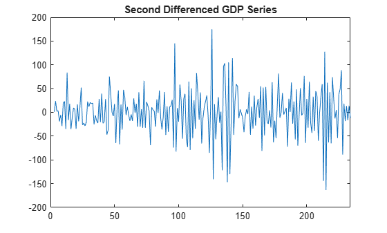
The second-differenced series appears more stationary.