Estimate Moving Average Trend Using Moving Average Filter
This example shows how to estimate long-term trend using a symmetric moving average function. This is a convolution that you can implement using conv. The time series is monthly international airline passenger counts from 1949 to 1960.
Load the airline data set (Data_Airline).
load Data_Airline
y = log(DataTimeTable.PSSG);
T = length(y);

figure
plot(DataTable.Time,y)
title("Log Airline Passenger Counts")
hold on
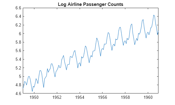
The data shows a linear trend and a seasonal component with periodicity 12.
The periodicity of the data is monthly, so a 13-term moving average is a reasonable choice for estimating the long-term trend. Use weight 1/24 for the first and last terms, and weight 1/12 for the interior terms. Add the moving average trend estimate to the observed time series plot.
wts = [1/24; repmat(1/12,11,1); 1/24];
yS = conv(y,wts,"valid");

h = plot(DataTimeTable.Time(7:end-6),yS,"r",LineWidth=2);
legend(h,"13-Term Moving Average")
hold off
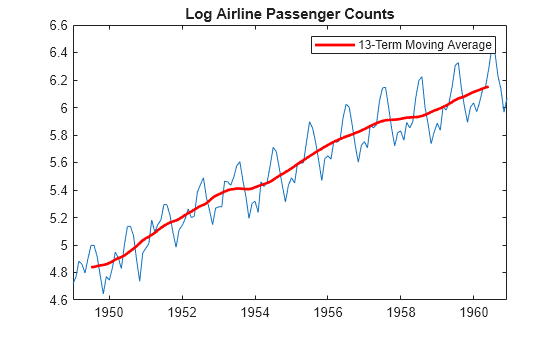
When you use the shape parameter "valid" in the call to conv, observations at the beginning and end of the series are lost. Here, the moving average has window length 13, so the first and last 6 observations do not have smoothed values.
What Is a Moving Average Filter?
Some time series are decomposable into various trend components. To estimate a trend component without making parametric assumptions, you can consider using a filter.
Filters are functions that transform one time series into another. By appropriate filter selection, certain patterns in the original time series can be clarified or eliminated in the new series. For example, a low-pass filter removes high frequency components, yielding an estimate of the slow-moving trend.
An example of a linear filter is the moving average. Consider a time series , . A symmetric (centered) moving average filter of window length is
You can choose any weights that sum to 1. To estimate a slow-moving trend, set for quarterly data (a 5-term moving average), or set for monthly data (a 13-term moving average). Because symmetric moving averages have an odd number of terms, a reasonable choice for the weights is for , and otherwise. Implement a moving average by convolving a time series with a vector of weights using the conv function.
You cannot apply a symmetric moving average to the q observations at the beginning and end of the series. This application results in observation loss. To preserve all observations, you can apply an asymmetric moving average at the ends of the series.
You can also select a web site from the following list:
Americas
- América Latina (Español)
- Canada (English)
- United States (English)
Europe
- Belgium (English)
- Denmark (English)
- Deutschland (Deutsch)
- España (Español)
- Finland (English)
- France (Français)
- Ireland (English)
- Italia (Italiano)
- Luxembourg (English)
- Netherlands (English)
- Norway (English)
- Österreich (Deutsch)
- Portugal (English)
- Sweden (English)
- Switzerland
- United Kingdom (English)