Estimate Vector Error-Correction Model Using Econometric Modeler
This example models the annual Canadian inflation and interest rate series by using the Econometric Modeler app. The example shows how to perform the following actions in the app:
Test each raw series for stationarity.
Test for cointegration and determine a Johansen cointegration form if cointegration is present.
Fit several completing vector error-correction (VEC) models, and choose the one with the best, parsimonious fit.
Diagnose each residual series.
Export the chosen model to the command line.
At the command line, the example uses the model to generate forecasts.
The data set, which is stored in Data_Canada, contains annual
Canadian inflation and interest rates from 1954 through 1994.
Load and Import Data into Econometric Modeler
At the command line, load the Data_Canada.mat data
set.
load Data_CanadaAt the command line, open the Econometric Modeler app.
econometricModeler
Alternatively, open the app from the apps gallery (see Econometric Modeler).
Import DataTimeTable into the app:
On the Modeler tab, in the Import section, click the Import button
 .
.In the Import Data dialog box, select the check box for the
DataTimeTablevariable.Click Import.
The Canadian interest and inflation rate variables appear in the Time Series pane, and a time series plot of all the series appears in the Plot(INF_C) figure window.

Plot only the three interest rate series INT_L,
INT_M, and INT_S
together. In the Time Series pane, click
INT_L and Ctrl+click
INT_M and INT_S. Then,
on the Plots tab, in the Plots
section, click Time Series. The time series plot
appears in the Plot(INT_L) document.
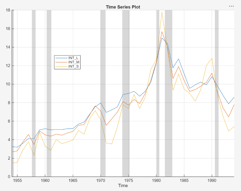
The interest rate series each appear nonstationary, and they appear to move together with mean-reverting spread. In other words, they exhibit cointegration. To establish these properties, this example conducts statistical tests.
Conduct Stationarity Test
Assess whether each interest rate series is stationary by conducting Phillips-Perron unit root tests. For each series, assume a stationary AR(1) process with drift for the alternative hypothesis. You can confirm this property by viewing the autocorrelation and partial autocorrelation function plots.
Close all plots in the right pane, and perform the following procedure for
each series INT_L, INT_M,
and INT_S.
In the Time Series pane, click a series.
On the Modeler tab, in the Tests section, click Add Test > Phillips-Perron Test.
On the PP tab, in the Settings section, in the Number of Lags box, type
1, and in the Model list select Autoregressive with Drift.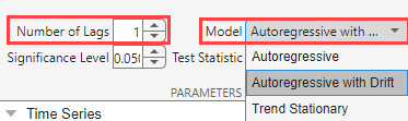
In the Tests section, click Run Test. Test results for the selected series appear in the PP(
series) tab.
Position the test results to view them simultaneously.
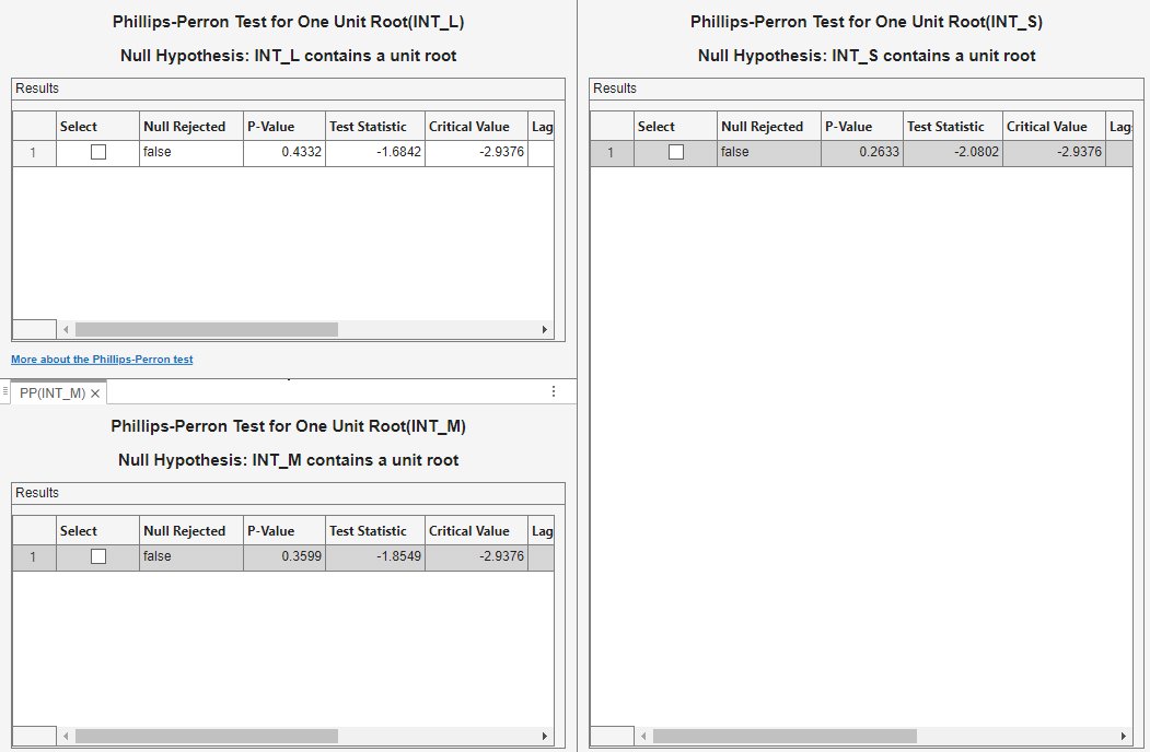
All tests fail to reject the null hypothesis that the series contains a unit root process.
Conduct Cointegration Test
To create and estimate a VEC model of unit root series, the series need to
exhibit cointegration. Conduct a Johansen test. Because the raw series do not
contain a linear trend, assume that the only deterministic term in the model is
an intercept in the cointegrating relation (H1*
Johansen form), and include 1 lagged difference term in the model.
In the Time Series pane, click
INT_Land Ctrl+clickINT_MandINT_S.In the Tests section, click Add Test > Johansen Test.
On the JCI tab, in the Settings section, in the Number of Lags box, type
1. In the Model list, select H1*.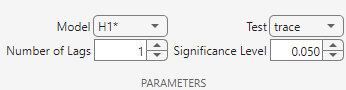
In the Tests section, click Run Test. Test results and a plot of the cointegration relation for the largest rank appear in the JCI tab.
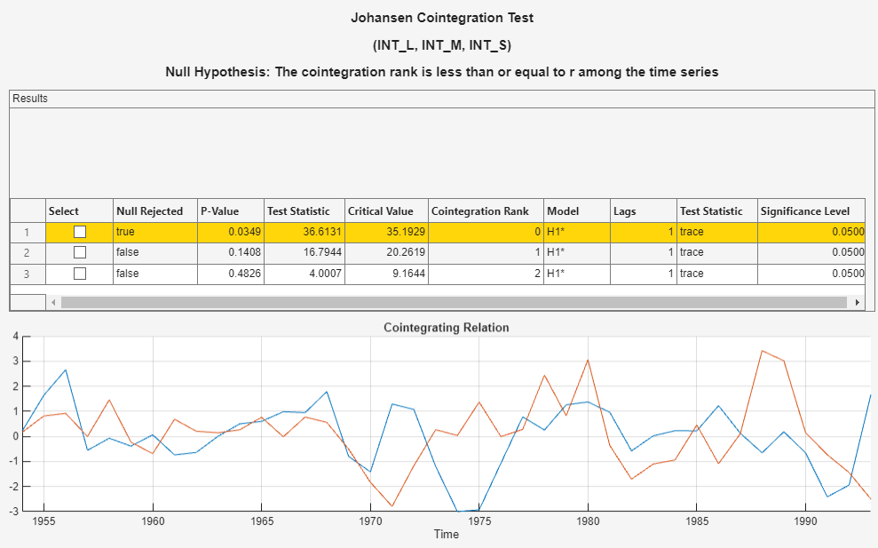
Econometric Modeler conducts a separate test for each cointegration rank 0 through 2 (the number of series – 1). The test rejects the null hypothesis of no cointegration (Cointegration rank = 0), but fails to reject the null hypothesis of Cointegration rank ≤ 1. The conclusion is to set the cointegration rank of the VEC model to 1.
Estimate VEC Models
Estimate 3-D VEC(p) models of the interest rate
series, with a cointegration rank of 1 and p = 1 and
2.
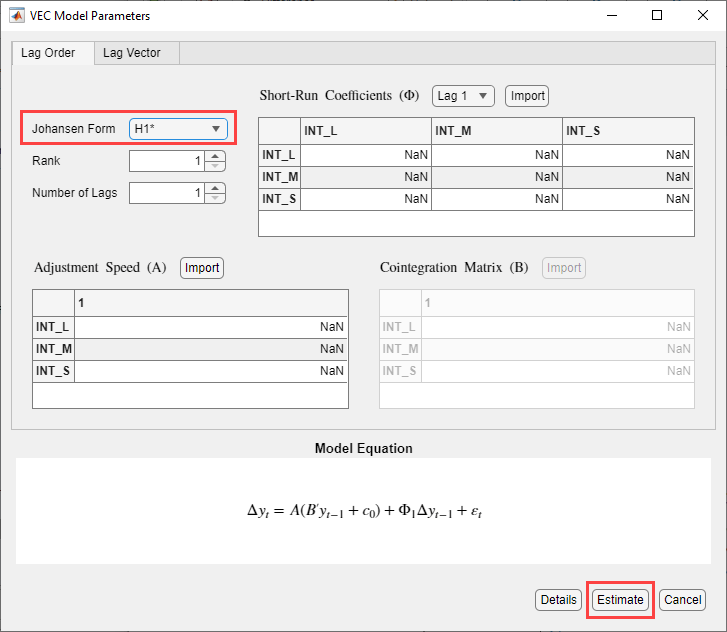
With
INT_L,INT_M, andINT_Sselected in the Time Series pane, in the Models section, click VEC.In the VEC Model Parameters dialog box, in the Johansen Form, select H1*. Fit the VEC(1) model by clicking Estimate.
The model variable
VECappears in the Models pane, its value appears in the Preview pane, and its estimation summary appears in the Fit(VEC) document. Change the name of theVECmodel toVEC_1by clickingVECtwice and then typingVEC_1.Repeat steps 1 and 2 for the short-run polynomial order
p= 2.Similar to the VEC(1) estimation, the variable
VEC_2appears in the Models pane, and its estimation summary appears in the Fit(VEC_2) tab. You can view properties of an estimated model in the Preview pane by clicking the model in the Models pane. For example, clickVEC.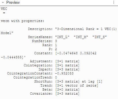
Select Model with Best In-Sample Fit
The estimation summary in each
Fit(VEC_p) tab contains a
plot of fitted values and residuals, with respect to the time series in the
Time Series list, a standard statistical table of
estimates and inferences, and a table of information criteria.
Compare the information criteria of each estimated model simultaneously by positioning the estimation summary documents so that they occupy the left and right sections of the right pane. The model with the lowest value has the best, parsimonious fit.
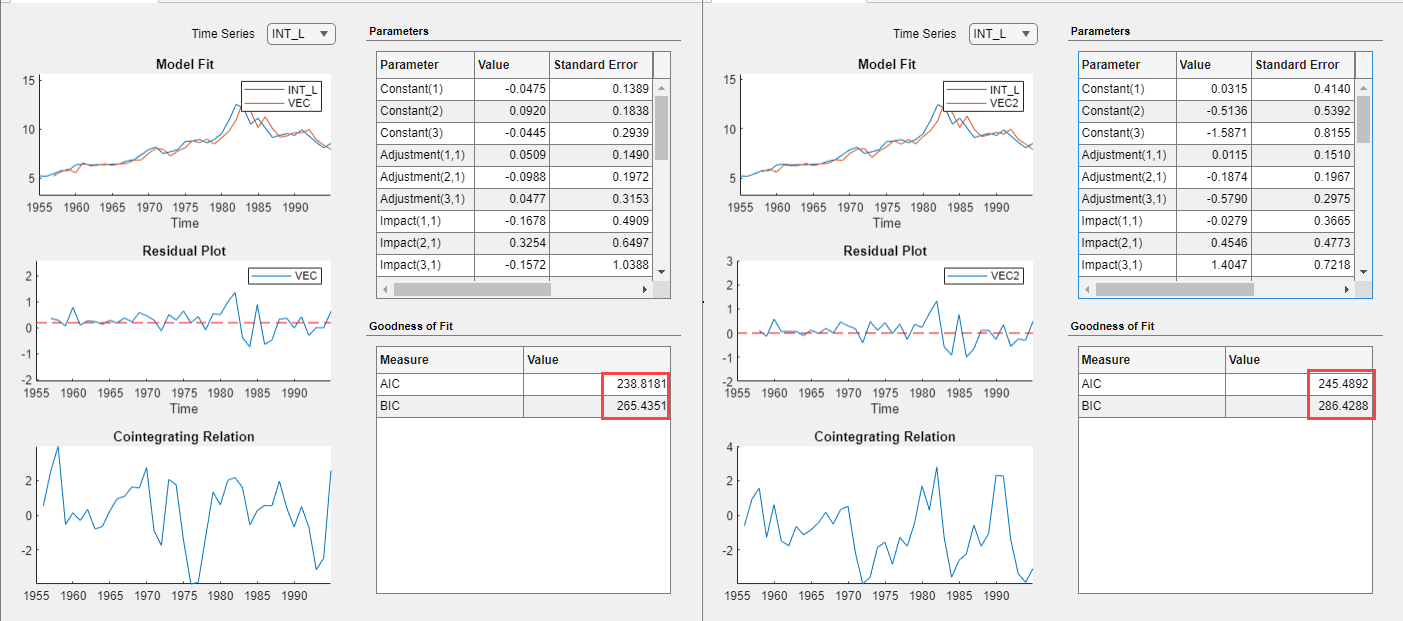
The VEC(1) model VEC produces the lowest AIC and
BIC values. Choose this model for further analysis.
Check Goodness of Fit
Inspect the following VEC(1) plots of each residual series:
Histograms, for center, normality, and outliers
Quantile-quantile plots, for normality, skewness, and tails
Autocorrelation function (ACF), for serial correlation
ACF of squared residual series, for heteroscedasticity
This example diagnoses the residuals visually. Alternatively, you can conduct statistical tests to diagnose the residuals.
Dismiss the Fit(VEC2) document by clicking ![]() on its tab.
on its tab.
On the Models pane, click
VEC_1.
Plot separate residual histograms. On the Modeler tab, in the Diagnostics section, click Model Fit Diagnostics > Residual Histogram. Histograms of the each residual series appear in the Hist(VEC_1) document.
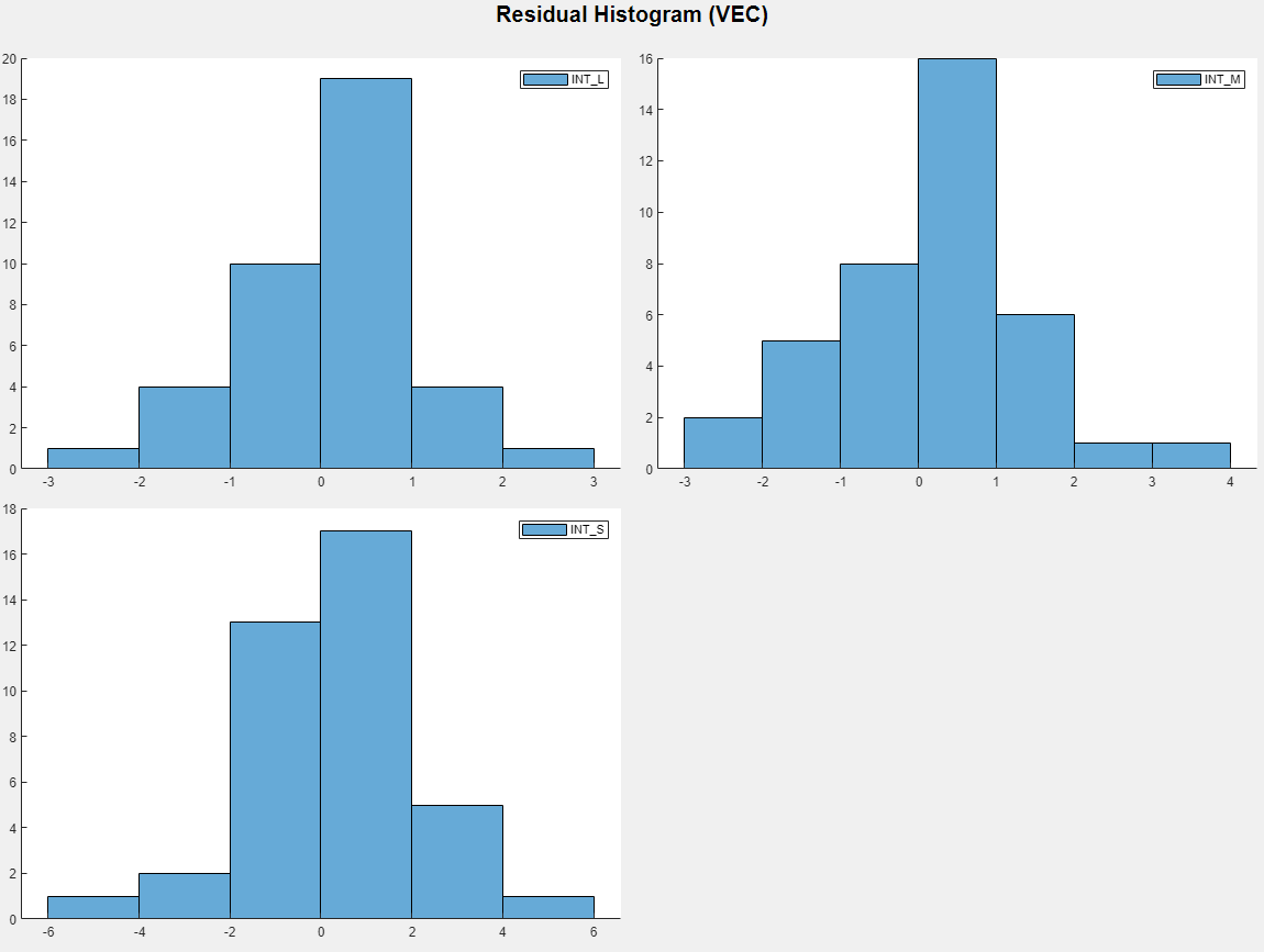
Each residual series appears approximately centered around 0 and approximately normal.
Plot separate residual quantile-quantile plots. With
VEC_1 selected in the Time
Series pane, on the Modeler tab, in the
Diagnostics section, click Model Fit
Diagnostics > Residual Q-Q Plot.
Quantile-quantile plots of each residual series appear in the
QQ(VEC_1) document.

The residual series are slightly skewed left and have lighter tails than the normal distribution. This example proceeds without addressing possible skewness and light tails.
Plot separate ACF plots of each residual series. With
VEC_1 selected in the Time
Series pane, on the Modeler tab, in the
Diagnostics section, click Model Fit
Diagnostics > Residual
Autocorrelation. ACF plots of each residual series appear in
the ACF(VEC_1) document.
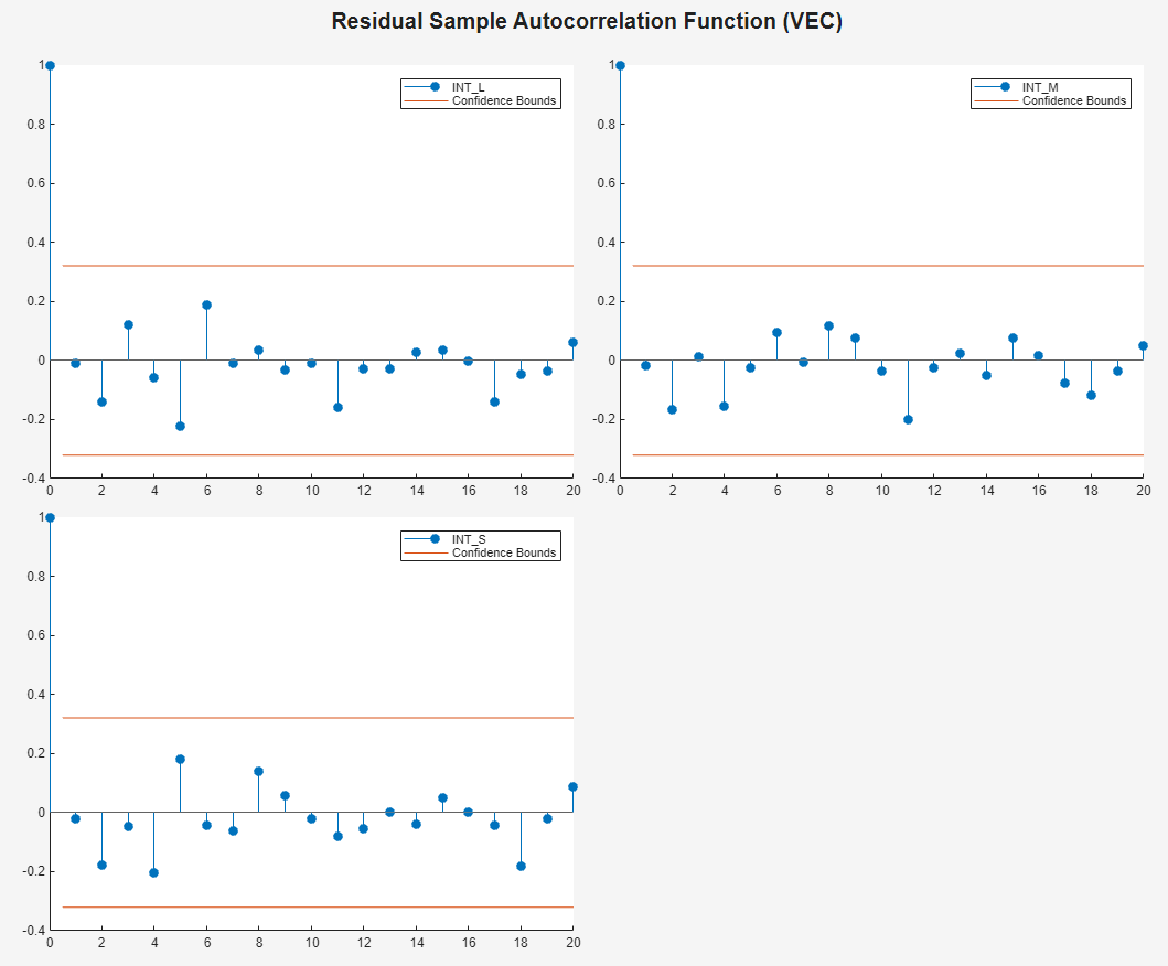
The residuals do not exhibit significant autocorrelation.
Plot separate ACF plots of each squared residual series. With
VEC_1 selected in the Time
Series pane, on the Modeler tab, in the
Diagnostics section, click Model Fit
Diagnostics > Squared Residual
Autocorrelation. ACF plots of each squared residual series
appear in the ACF(VEC_1)_2 document.

Each squared residual series has significant autocorrelations at early lags, which suggests that heteroscedasticity is present in all series. This example proceeds without addressing possible heteroscedasticity.
Generate Forecasts
Generate MMSE forecasts and approximate 95% forecast intervals from the estimated VEC(1) model for the next four years (16 quarters).
In the Models pane, select the
VEC_1model.In the Modeler tab, in the Forecast section, click Forecast.
In the Forecast Model Response dialog box, set Number of periods in forecast horizon to
16. Then, click Forecast.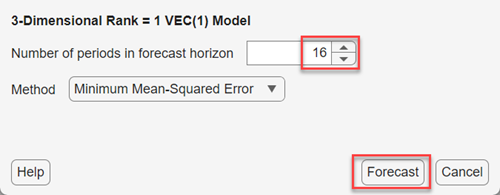
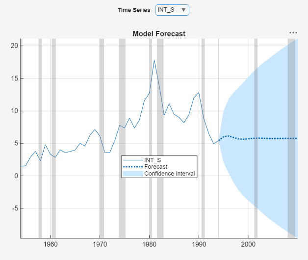
In the right pane, in the For(VEC_1) tab is a figure
window of a plot of the INT_L series with forecasts
and 95% forecast intervals at the end of the series, generated from the VEC(1)
model.

To display the forecasts of the other variables in the VEC(1) model, use the
Time Series menu in the figure window. For example,
display the forecasts of the INT_S series, in the
figure window, click Time Series >
INT_S.