Create ARIMA Models That Include Exogenous Covariates
These examples show how to create various ARIMAX models by using the
arima function.
Create ARIMAX Model Using Longhand Syntax
This example shows how to specify an ARIMAX model using longhand syntax.
Specify the ARIMAX(1,1,0) model that includes three predictors:
Mdl = arima('AR',0.1,'D',1,'Beta',[3 -2 5])
Mdl =
  arima with properties:

     Description: "ARIMAX(1,1,0) Model (Gaussian Distribution)"
      SeriesName: "Y"
    Distribution: Name = "Gaussian"
               P: 2
               D: 1
               Q: 0
        Constant: NaN
              AR: {0.1} at lag [1]
             SAR: {}
              MA: {}
             SMA: {}
     Seasonality: 0
            Beta: [3 -2 5]
        Variance: NaN
The output shows that the ARIMAX model Mdl has the following qualities:
Property
Pin the output is the sum of the autoregressive lags and the degree of integration, i.e.,P=p+D=2.Betacontains three coefficients corresponding to the effect that the predictors have on the response.Mdldoes not store predictor or response data. You specify the required data when you operate onMdl.The rest of the properties are 0,
NaN, or empty cells.
Be aware that if you specify nonzero D or Seasonality, then Econometrics Toolbox™ differences the response series before the predictors enter the model. Therefore, the predictors enter a stationary model with respect to the response series . You should preprocess the predictors by testing for stationarity and differencing if any are unit root nonstationary. If any nonstationary predictor enters the model, then the false negative rate for significance tests of can increase.
Specify ARMAX Model Using Dot Notation
This example shows how to specify a stationary ARMAX model using arima.
Specify the ARMAX(2,1) model
by including one stationary exogenous covariate in arima.
Mdl = arima('AR',[0.2 -0.3],'MA',0.1,'Constant',6,'Beta',3)
Mdl =
  arima with properties:

     Description: "ARIMAX(2,0,1) Model (Gaussian Distribution)"
      SeriesName: "Y"
    Distribution: Name = "Gaussian"
               P: 2
               D: 0
               Q: 1
        Constant: 6
              AR: {0.2 -0.3} at lags [1 2]
             SAR: {}
              MA: {0.1} at lag [1]
             SMA: {}
     Seasonality: 0
            Beta: [3]
        Variance: NaN
The output shows the model Mdl has NaN values or an empty cell ({}) for the Variance, SAR, and SMA properties. You can modify the model using dot notation at the command line. For example, you can introduce another exogenous, stationary covariate, and specify the variance of the innovations as 0.1
Modify the model by specifying an innovations variance of 0.1 and regression coefficient values.
Mdl.Beta = [3 -2];
Mdl.Variance = 0.1;
Mdl
Mdl =
  arima with properties:

     Description: "ARIMAX(2,0,1) Model (Gaussian Distribution)"
      SeriesName: "Y"
    Distribution: Name = "Gaussian"
               P: 2
               D: 0
               Q: 1
        Constant: 6
              AR: {0.2 -0.3} at lags [1 2]
             SAR: {}
              MA: {0.1} at lag [1]
             SMA: {}
     Seasonality: 0
            Beta: [3 -2]
        Variance: 0.1
Specify ARIMAX or SARIMAX Model Using Econometric Modeler App
In the Econometric Modeler app, you can specify the seasonal and nonseasonal lag structure, presence of a constant, innovation distribution, and predictor variables of an ARIMA(p,D,q) or a SARIMA(p,D,q)×(ps,Ds,qs)s model by following these steps. All specified coefficients are unknown but estimable parameters.
At the command line, open the Econometric Modeler app.
econometricModeler
Alternatively, open the app from the apps gallery (see Econometric Modeler).
In the Time Series pane, select the response time series to which the model will be fit.
On the Econometric Modeler tab, in the Models section, click the arrow to display the models gallery. For strictly nonseasonal models, click ARIMAX; for seasonal models, click SARIMAX. ARIMAX and SARIMAX models must contain at least one predictor variable.
The
TypeModel Parameters dialog box appears. This figure shows the SARIMAX Model Parameters dialog box. All variables in the Time Series pane, except the chosen response variable, appear in the Predictors section.
Specify the lag structure. Use the Lag Order tab to specify a model that includes:
All consecutive lags from 1 through their respective orders, in the seasonal polynomials
Lags that are all consecutive multiples of the period (s), in the seasonal polynomials
An s-degree seasonal integration polynomial
For the flexibility to specify the inclusion of particular lags, use the Lag Vector tab. For more details, see Specifying Univariate Lag Operator Polynomials Interactively. Regardless of the tab you use, you can verify the model form by inspecting the equation in the Model Equation section.
In the Predictors section, choose at least one predictor variable by selecting the Include? check box for the time series.
For example, suppose you are working with the
Data_USEconModel.mat data set and its variables are listed in
the Time Series pane.
To specify an ARIMAX(3,1,2) model for the unemployment rate containing a constant, all consecutive AR and MA lags from 1 through their respective orders, Gaussian-distributed innovations, and the predictor variables COE, CPIAUCSL, FEDFUNDS, and GDP:
In the Time Series pane, select the
UNRATEtime series.On the Econometric Modeler tab, in the Models section, click the arrow to display the models gallery.
In the models gallery, in the ARMA/ARIMA Models section, click ARIMAX.
In the ARIMAX Model Parameters dialog box in the Nonseasonal section of the Lag Order tab, set Degree of Integration to
1.Set Autoregressive Order to
3.Set Moving Average Order to
2.In the Predictors section, select the Include? check box for the COE, CPIAUCSL, FEDFUNDS, and GDP time series.
To specify an ARIMAX(3,1,2) model for the unemployment rate containing all AR and MA lags from 1 through their respective orders, Gaussian-distributed innovations, no constant, and the predictor variables COE and CPIAUCSL:
In the Time Series pane, select the
UNRATEtime series.On the Econometric Modeler tab, in the Models section, click the arrow to display the models gallery.
In the models gallery, in the ARMA/ARIMA Models section, click ARIMAX.
In the ARIMAX Model Parameters dialog box, in the Nonseasonal section of the Lag Order tab, set Degree of Integration to
1.Set Autoregressive Order to
3.Set Moving Average Order to
2.Clear the Include Constant Term check box.
In the Predictors section, select the Include? check box for the COE and CPIAUCSL time series.
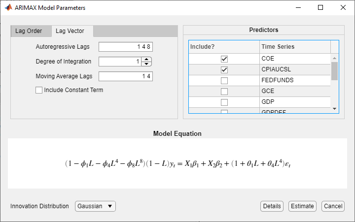
To specify an ARMA(8,1,4) model for the unemployment rate containing nonconsecutive lags
where εt is a series of IID Gaussian innovations:
In the Time Series pane, select the
UNRATEtime series.On the Econometric Modeler tab, in the Models section, click the arrow to display the models gallery.
In the models gallery, in the ARMA/ARIMA Models section, click ARIMAX.
In the ARIMAX Model Parameters dialog box, click the Lag Vector tab.
Set Degree of Integration to
1.Set Autoregressive Lags to
1 4 8.Set Moving Average Lags to
1 4.Clear the Include Constant Term check box.
In the Predictors section, select the Include? check box for the COE and CPIAUCSL time series.
To specify an ARIMA(3,1,2) model for the unemployment rate containing all consecutive AR and MA lags through their respective orders, a constant term, the predictor variables COE and CPIAUCSL, and t-distributed innovations:
In the Time Series pane, select the
UNRATEtime series.On the Econometric Modeler tab, in the Models section, click the arrow to display the models gallery.
In the models gallery, in the ARMA/ARIMA Models section, click ARIMAX.
In the ARIMAX Model Parameters dialog box, in the Nonseasonal section of the Lag Order tab, set Degree of Integration to
1.Set Autoregressive Order to
3.Set Moving Average Order to
2.Click the Innovation Distribution button, then select
t.In the Predictors section, select the Include? check box for COE and CPIAUCSL time series.
The degrees of freedom parameter of the t distribution is an unknown but estimable parameter.
After you specify a model, click Estimate to estimate all unknown parameters in the model.
What Are ARIMA Models That Include Exogenous Covariates?
ARIMAX(p,D,q) Model
The autoregressive moving average model including exogenous covariates, ARMAX(p,q), extends the ARMA(p,q) model by including the linear effect that one or more exogenous series has on the stationary response series yt. The general form of the ARMAX(p,q) model is
| (1) |
| (2) |
You can use this model to check if a set of exogenous variables has an effect on a linear time series. For example, suppose you want to measure how the previous week’s average price of oil, xt, affects this week’s United States exchange rate yt. The exchange rate and the price of oil are time series, so an ARMAX model can be appropriate to study their relationships.
Conventions and Extensions of the ARIMAX Model
ARMAX models have the same stationarity requirements as ARMA models. Specifically, the response series is stable if the roots of the homogeneous characteristic equation of lie outside of the unit circle according to Wold’s Decomposition [2].
If the response series yt is not stable, then you can difference it to form a stationary ARIMA model. Do this by specifying the degrees of integration
D. Econometrics Toolbox™ enforces stability of the AR polynomial. When you specify an AR model usingarima, the software displays an error if you enter coefficients that do not correspond to a stable polynomial. Similarly,estimateimposes stationarity constraints during estimation.The software differences the response series yt before including the exogenous covariates if you specify the degree of integration
D. In other words, the exogenous covariates enter a model with a stationary response. Therefore, the ARIMAX(p,D,q) model is
where c* = c/(1 – L)D and θ*(L) = θ(L)/(1 – L)D. Subsequently, the interpretation of β has changed to the expected effect a unit increase in the predictor has on the difference between current and lagged values of the response (conditional on those lagged values).(3) You should assess whether the predictor series xt are stationary. Difference all predictor series that are not stationary with
diffduring the data preprocessing stage. If xt is nonstationary, then a test for the significance of β can produce a false negative. The practical interpretation of β changes if you difference the predictor series.The software uses maximum likelihood estimation for conditional mean models such as ARIMAX models. You can specify either a Gaussian or Student’s t for the distribution of the innovations.
You can include seasonal components in an ARIMAX model (see What Are Multiplicative ARIMA Models?) which creates a SARIMAX(p,D,q)(ps,Ds,qs)s model. Assuming that the response series yt is stationary, the model has the form
where Φ(L) and Θ(L) are the seasonal lag polynomials. If yt is not stationary, then you can specify degrees of nonseasonal or seasonal integration using
arima. If you specifySeasonality≥ 0, then the software applies degree one seasonal differencing (Ds = 1) to the response. Otherwise, Ds = 0. The software includes the exogenous covariates after it differences the response.The software treats the exogenous covariates as fixed during estimation and inference.
References
[1] Box, George E. P., Gwilym M. Jenkins, and Gregory C. Reinsel. Time Series Analysis: Forecasting and Control. 3rd ed. Englewood Cliffs, NJ: Prentice Hall, 1994.
[2] Wold, Herman. "A Study in the Analysis of Stationary Time Series." Journal of the Institute of Actuaries 70 (March 1939): 113–115. https://doi.org/10.1017/S0020268100011574.
See Also
Apps
Objects
Functions
Related Topics
- Estimate ARIMAX Model Using Econometric Modeler App
- Analyze Time Series Data Using Econometric Modeler
- Specifying Univariate Lag Operator Polynomials Interactively
- Forecast IGD Rate from ARX Model
- Modify Properties of Conditional Mean Model Objects
- Specify ARMAX Model Using Dot Notation
- Create ARIMAX Model Using Longhand Syntax
You can also select a web site from the following list:
Americas
- América Latina (Español)
- Canada (English)
- United States (English)
Europe
- Belgium (English)
- Denmark (English)
- Deutschland (Deutsch)
- España (Español)
- Finland (English)
- France (Français)
- Ireland (English)
- Italia (Italiano)
- Luxembourg (English)
- Netherlands (English)
- Norway (English)
- Österreich (Deutsch)
- Portugal (English)
- Sweden (English)
- Switzerland
- United Kingdom (English)