Simulink Simulation of Deep Learning Models Using MATLAB Function Block

Since R2025a

This example shows to how to predict responses for a pretrained long short-term memory (LSTM) network by using a MATLAB® Function block in Simulink®.

Load Pretrained Network

Load JapaneseVowelsNet, a pretrained LSTM network trained on the Japanese vowels data set described in [1] and [2]. This network was trained on the sequences sorted by sequence length with a mini-batch size of 27. To learn about the network and the network training process, see Train Network Using Custom Mini-Batch Datastore for Sequence Data (Deep Learning Toolbox).

load JapaneseVowelsDlnet.mat

View the network architecture.

analyzeNetwork(dlnet);

Load Test Data

Load the Japanese vowels test data. XTest is a cell array that contains 370 sequences of dimension 12 of varying length. The data are categorized into nine classes, which correspond to the nine speakers. TTest is a categorical vector of labels, "1","2",..."9".

Create a timetable array named simin with time-stamped rows and multiple copies of X.

load JapaneseVowelsTestData
X = XTest{94};
numTimeSteps = size(X,2);
simin = timetable(repmat(X,1,4)','TimeStep',seconds(0.2));

Open Simulink Model

Open the StatefulPredictMLFBExample model. This model contains a MATLAB Function block that predicts the scores and From Workspace block that loads the input data sequence over the time steps.

open_system('StatefulPredictMLFBExample');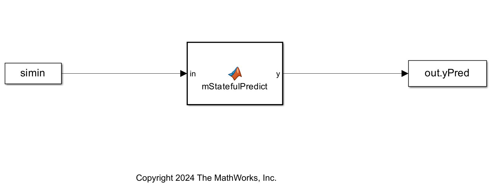

Examine the MATLAB Function Block

The MATLAB Function block named mStatefulPredict outputs the prediction scores. In the model, double-click the MATLAB Function block to see the code. The function uses a persistent variable to hold the dlnetwork and its State and then:

1. Uses the coder.load function to load a MAT file that contains the dlnetwork object.

2. Converts the input into a formatted dlarray object by specifying the format as 'CT', where 'C' is the 'Channel' and 'T' is 'Time'.

3. Calls the predict function by passing the dlnetwork and the input. The predict function returns the predicted scores and the updated state of the network.

4. Updates the State property of the dlnetwork object with the new state.

5. Extracts the raw data from the predicted output and returns it as the output of the MATLAB Function block.

function y = mStatefulPredict(in)

% Create a persistent variable named 'S' that contains the dlnetwork as a
% field. Upon subsequent calls to mStatefulPredict function, the persisent
% variable's State is internally updated without have to return it out of
% the function.
persistent S
if isempty(S)
    S = coder.load("JapaneseVowelsDlnet.mat");
end

% Create a labelled dlarray object to invoke predict on the dlnetwork
dlIn = dlarray(in, 'CT');
[dlOut, state] = predict(S.dlnet, single(dlIn));

% Update the state of the dlnetwork
S.dlnet.State = state;

% Extract the data from the dlarray object to return it out
y = double(extractdata(dlOut));

end

Run the Simulation

To compute responses for the pretrained LSTM network, run the simulation. The model saves the prediction scores prediction scores in the MATLAB workspace.

out = sim('StatefulPredictMLFBExample');

Run Simulation by Using Rapid Accelerator Mode

You can simulate the model model in accelerator and rapid accelerator modes. To enable rapid accelerator mode, set the SimulationMode parameter value of the model to "rapid-accelerator".

out = sim('StatefulPredictMLFBExample', SimulationMode = "rapid-accelerator");

### Searching for referenced models in model 'StatefulPredictMLFBExample'.
### Total of 1 models to build.
### Building the rapid accelerator target for model: StatefulPredictMLFBExample
### Successfully built the rapid accelerator target for model: StatefulPredictMLFBExample

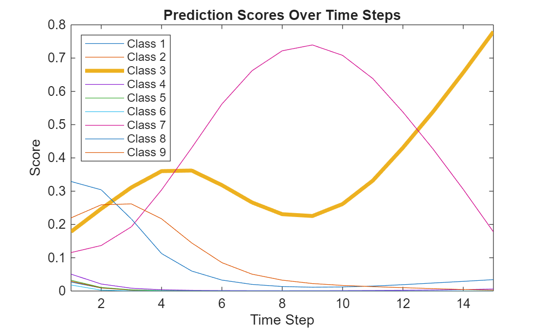
Plot how the prediction scores change between time steps.

scores = squeeze(out.yPred.Data(:,:,1:numTimeSteps));

classNames = string(1:9);
figure
lines = plot(scores');
xlim([1 numTimeSteps])
legend("Class " + classNames,'Location','northwest')
xlabel("Time Step")
ylabel("Score")
title("Prediction Scores Over Time Steps")

Highlight the prediction scores over time steps for the true class.

trueLabel = TTest(94);
lines(trueLabel).LineWidth = 3;

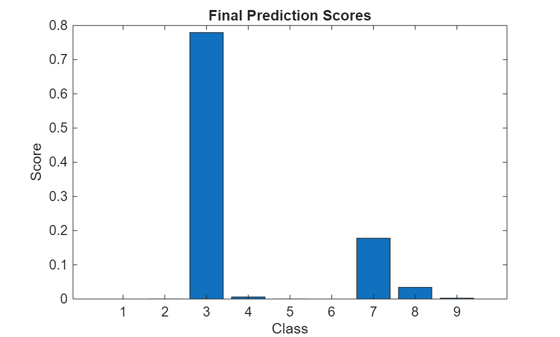
Display the final time step prediction in a bar chart.

figure
bar(scores(:,end))
title("Final Prediction Scores")
xlabel("Class")
ylabel("Score")

References

[1] M. Kudo, J. Toyama, and M. Shimbo. "Multidimensional Curve Classification Using Passing-Through Regions." Pattern Recognition Letters. Vol. 20, No. 11–13, pages 1103–1111.

[2] UCI Machine Learning Repository: Japanese Vowels Dataset. https://archive.ics.uci.edu/ml/datasets/Japanese+Vowels