Design Lowpass FIR Filters
This example shows how to design lowpass FIR filters. You can extend many of the concepts presented here to other responses such as highpass, bandpass, and others.
FIR filters are widely used because of the powerful design algorithms that exist to design such filters. These filters are also inherently stable when implemented in the nonrecursive form, and you can easily attain linear phase and also extend them to multirate cases, and there is ample hardware support for these filters. This example showcases functions and objects from DSP System Toolbox™ that you can use to design lowpass FIR filters.
Obtain Lowpass FIR Filter Coefficients
The Lowpass Filter Design in MATLAB example highlights some of the commonly used command-line tools in DSP System Toolbox to design lowpass filters. This example provides a more comprehensive overview of the design options available in the toolbox for designing lowpass filters. To begin with, this example presents two functions that return a vector of FIR filter coefficients: firceqrip and firgr. Use firceqrip when the filter order (equivalently the filter length) is known and fixed.
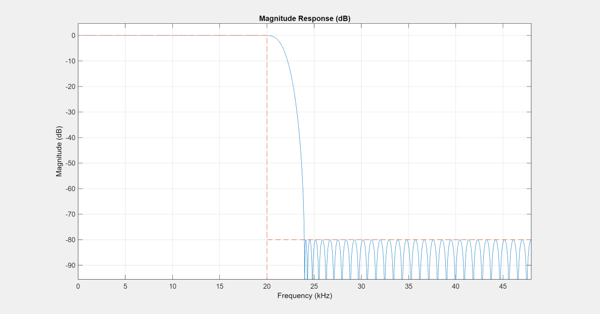
N   = 100;        % FIR filter order
Fp  = 20e3;       % 20 kHz passband-edge frequency
Fs  = 96e3;       % 96 kHz sampling frequency
Rp  = 0.00057565; % Corresponds to 0.01 dB peak-to-peak ripple
Rst = 1e-4;       % Corresponds to 80 dB stopband attenuation

eqnum = firceqrip(N,Fp/(Fs/2),[Rp Rst],'passedge'); % eqnum = vec of coeffs
filterAnalyzer(eqnum,SampleRate=Fs) % Visualize filter
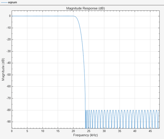
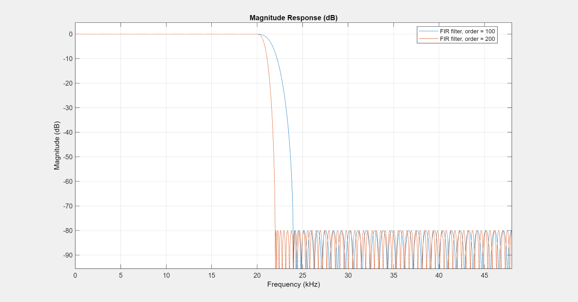
You set the filter order arbitrarily to 100 in the previous step. In general, a larger order results in a better approximation of the ideal filter at a high implementation cost. Double the filter order to reduce the transition width of the filter by half (keeping all other parameters the same).
N2 = 200; % Change filter order from 100 to 200
eqNum200 = firceqrip(N2,Fp/(Fs/2),[Rp Rst],'passedge');
fvt = filterAnalyzer(eqnum,1,eqNum200,1,SampleRate=Fs);
setLegendStrings(fvt, "FIR filter, order = "+[N N2])
Minimum-Order Lowpass Filter Design
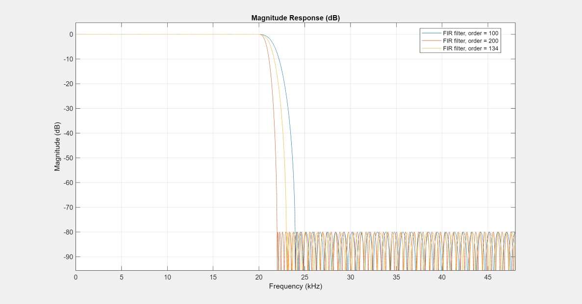
Instead of specifying the filter order, you can use firgr to determine the minimum order required to meet the design specifications. In order to do so, specify the width of the transition region by setting the stopband edge frequency.
Fst = 23e3;  % Transition Width = Fst - Fp
numMinOrder = firgr('minorder',[0,Fp/(Fs/2),Fst/(Fs/2),1],[1 1 0 0],...
    [Rp Rst]);
fvt = filterAnalyzer(eqnum,1,eqNum200,1,numMinOrder,1,SampleRate=Fs);
setLegendStrings(fvt,"FIR filter, order = "+[N N2 numel(numMinOrder)])
You can also use the firgr function to design even ('mineven') or odd ('minodd') minimum order filters.
Implement Lowpass FIR Filter
Once you obtain the filter coefficients, you can implement the filter using the dsp.FIRFilter System object™. The System object supports double/single precision floating-point data as well as fixed-point data. It also supports C and HDL code generation as well as optimized code generation for ARM® Cortex® M and ARM Cortex A.
lowpassFIR = dsp.FIRFilter(Numerator=eqnum); %or eqNum200 or numMinOrder
filterAnalyzer(lowpassFIR,SampleRate=Fs)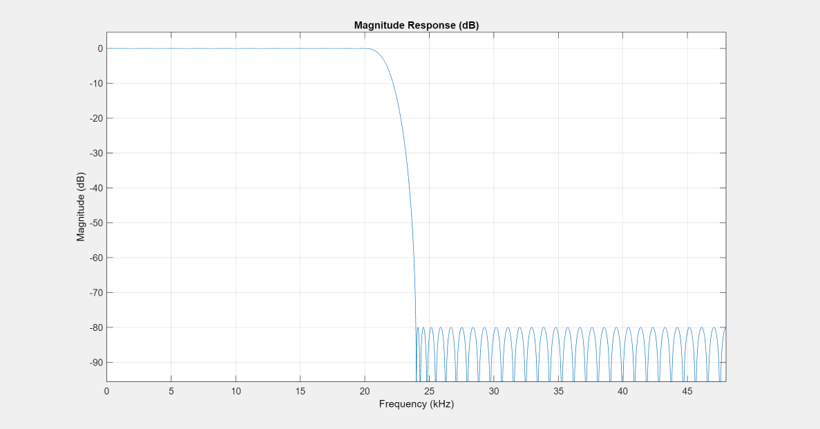
In order to perform the actual filtering, call the dsp.FIRFilter object directly like a function. This code filters Gaussian white noise and shows the resulting filtered signal in the spectrum analyzer for 10 seconds.
scope  = spectrumAnalyzer(SampleRate=Fs,AveragingMethod='exponential',ForgettingFactor=0.5);
show(scope);
tic
while toc < 10
    x = randn(256,1);
    y = lowpassFIR(x);
    scope(y);
end
Design and Implement Filter in One Step
You can also design and implement filter in a single step using the dsp.LowpassFilter System object. This System object also supports floating-point, fixed-point, C code generation, and ARM Cortex M and ARM Cortex A optimizations.
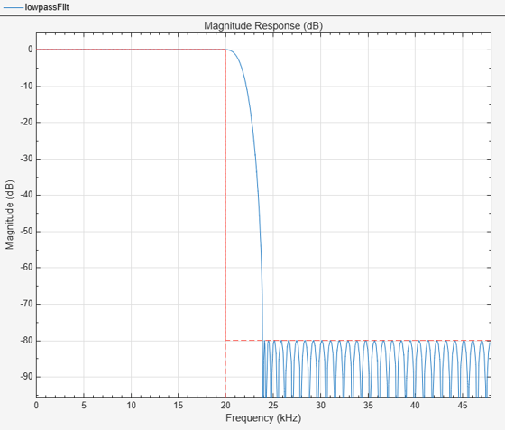
lowpassFilt = dsp.LowpassFilter(DesignForMinimumOrder=false, ...
    FilterOrder=N,PassbandFrequency=Fp,SampleRate=Fs,...
    PassbandRipple=0.01, StopbandAttenuation=80);
tic
while toc < 10
    x = randn(256,1);
    y = lowpassFilt(x);
    scope(y);
end
The System object expresses the filter magnitude in dB. To examine the passband ripple, use Filter Analyzer
filterAnalyzer(lowpassFilt)
Obtain Filter Coefficients
Extract the filter coefficients from the System object by using the tf function.
eqnum = tf(lowpassFilt);
Tunable Lowpass FIR Filters
To implement lowpass FIR filters in which you can tune the cutoff frequency at run-time, use the dsp.VariableBandwidthFIRFilter object. These filters do not provide the same granularity of control over the response characteristics of the filter, but they do allow for a dynamic frequency response.
vbwFilter = dsp.VariableBandwidthFIRFilter(CutoffFrequency=1e3);
tic
told = 0;
while toc < 10
    t = toc;
    if floor(t) > told
        % Add 1 kHz every second
        vbwFilter.CutoffFrequency = vbwFilter.CutoffFrequency + 1e3;
    end
    x = randn(256,1);
    y = vbwFilter(x);
    scope(y);
    told = floor(t);
end
Advanced Design Options: Optimal Nonequiripple Lowpass Filters
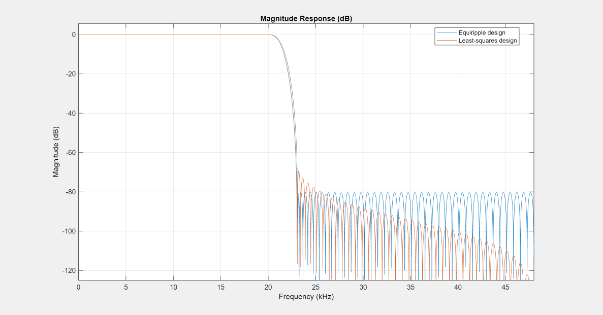
This example has so far discussed optimal equiripple designs. Equiripple designs achieve optimality by distributing the deviation from the ideal response uniformly. These designs have the advantage of minimizing the maximum deviation (ripple). However, the overall deviation, measured in terms of its energy tends to be large, which might not be desirable always. When you lowpass filter a signal, the remnant energy of the signal in the stopband can be relatively large. When this is a concern, the least-squares methods provide optimal designs that minimize the energy in the stopband. You can use the lowpassfir response in designfilt to design least-squares and other lowpass filters. Compare a least-squares FIR design to an FIR equiripple design with the same filter order and transition width.
lsFIR = designfilt("lowpassfir",FilterOrder=133,PassbandFrequency=Fp,StopBandFrequency=Fst, ...
    DesignMethod="ls",SampleRate=Fs,SystemObject=true);
LP_MIN = dsp.FIRFilter(Numerator=numMinOrder);
fvt = filterAnalyzer(LP_MIN,lsFIR.tf,SampleRate=Fs);
setLegendStrings(fvt,["Equiripple design","Least-squares design"])
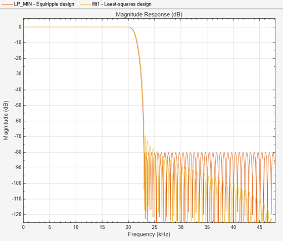
The attenuation in the stopband increases with frequency in the least-squares design, while it remains constant in the equiripple design. The increased attenuation in the least-squares case minimizes the energy in the band in which you filter the signal.
Equiripple Designs with Increasing Stopband Attenuation
An often undesirable effect of least-squares designs is that the ripple in the passband region close to the passband edge tends to be large. For lowpass filters in general, it is desirable that passband frequencies of a signal that you want to filter are affected as little as possible. To this extent, an equiripple passband is generally preferred. If you still want to have an increasing attenuation in the stopband, equiripple design options provide a way to achieve that.
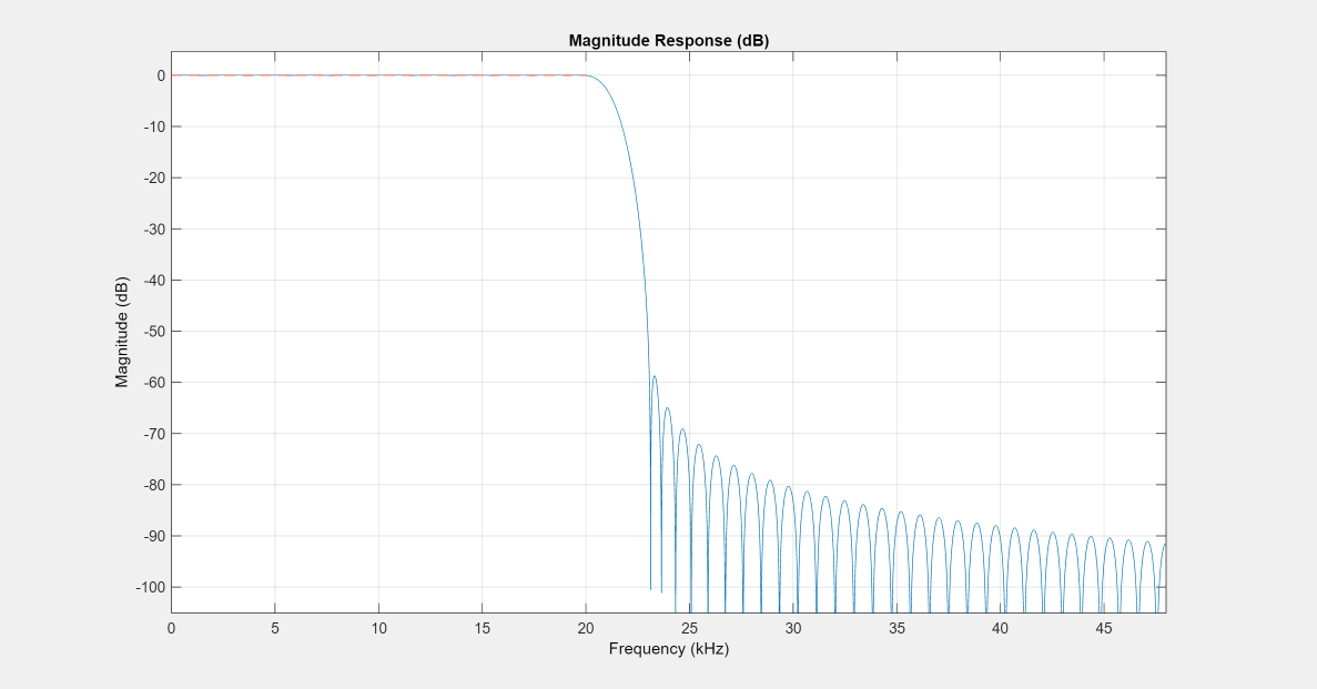
FIR_eqrip_slope = designfilt("lowpassfir",FilterOrder=133,PassbandFrequency=Fp,StopBandFrequency=Fst, ...
    DesignMethod="equiripple",SampleRate=Fs,StopbandShape="1/f",StopbandDecay=4,SystemObject=true);
fvt = filterAnalyzer(lsFIR,FIR_eqrip_slope);
setLegendStrings(fvt,["Least-squares design",...
    "Equiripple design with stopband decaying as (1/f)^4"])
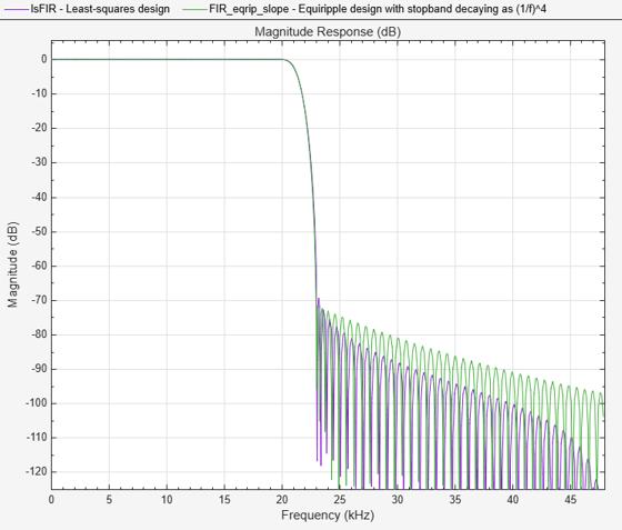
The stopbands in the two designs are quite similar. However, the equiripple design has a significantly smaller passband ripple in the vicinity of the passband-edge frequency of 20 kHz.
mls = measure(lsFIR);
meq = measure(FIR_eqrip_slope);
mls.Apass
ans =
0.0121
meq.Apass
ans =
0.0046
You can also implement increasing stopband attenuation by using an arbitrary magnitude specification and selecting two bands (one for the passband and one for the stopband). Then, by using weights for the second band, you can increase the attenuation throughout the band. For more information on this and other arbitrary magnitude designs, see Arbitrary Magnitude Filter Design.
B   = 2; % Number of bands
F   = [0 Fp linspace(Fst,Fs/2,40)];
A   = [1 1 zeros(1,length(F)-2)];
W   = linspace(1,100,length(F)-2);
lpfilter = designfilt("arbmagfir",FilterOrder=N,NumBands=B, ...
    BandFrequencies1=F(1:2),BandAmplitudes1=A(1:2), ...
    BandFrequencies2=F(3:end),BandAmplitudes2=A(3:end), ...
    BandWeights2=W,SampleRate=Fs, ...
    DesignMethod="equiripple",SystemObject=true);
filterAnalyzer(lpfilter);
Minimum-Phase Lowpass Filter Design
This example has so far only considered linear-phase designs. Linear phase is desirable in many applications. Nevertheless, if linear phase is not a requirement, minimum-phase designs can provide significant improvements over the linear phase counterparts. However, minimum-phase designs are not always numerically robust. Always check your design in Filter Analyzer.
Compare a linear-phase design with a minimum-phase design that meets the same design specifications to illustrate the advantages of minimum-phase design.
Fp  = 20e3;
Fst = 22e3;
Fs  = 96e3;
Ap  = 0.06;
Ast = 80;

linphaseSpec = designfilt("lowpassfir",PassbandFrequency=Fp,StopbandFrequency=Fst, ...
    PassbandRipple=Ap,StopbandAttenuation=Ast,SampleRate=Fs, ...
    DesignMethod="equiripple",SystemObject=true);

eqripSpec = designfilt("lowpassfir",PassbandFrequency=Fp,StopbandFrequency=Fst, ...
    PassbandRipple=Ap,StopbandAttenuation=Ast,SampleRate=Fs, ...
    DesignMethod="equiripple",PhaseConstraint="minimum",SystemObject=true);

fvt = filterAnalyzer(linphaseSpec,eqripSpec);
setLegendStrings(fvt,...
    ["Linear-phase equiripple design",...
    "Minimum-phase equiripple design"])
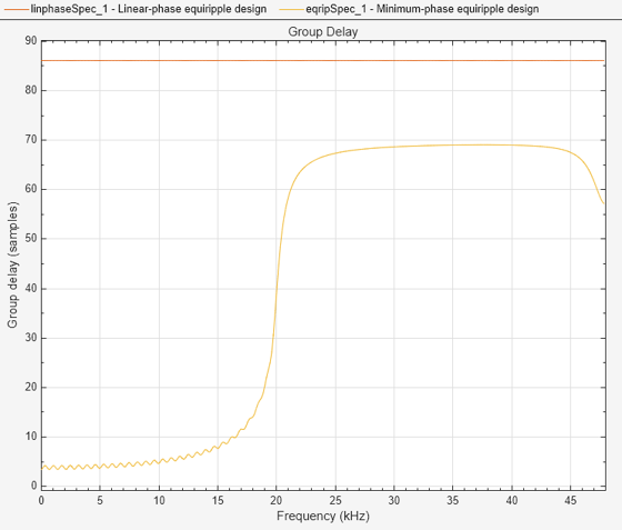
The number of coefficients have reduced from 173 to 141. Create a group delay plot and observe how the group delay is much smaller (in particular in the passband region).
fvt = filterAnalyzer(linphaseSpec,eqripSpec,...
    Analysis='groupdelay');
setLegendStrings(fvt,...
    ["Linear-phase equiripple design",...
    "Minimum-phase equiripple design"])
Minimum-Order Lowpass Filter Design Using Multistage Techniques
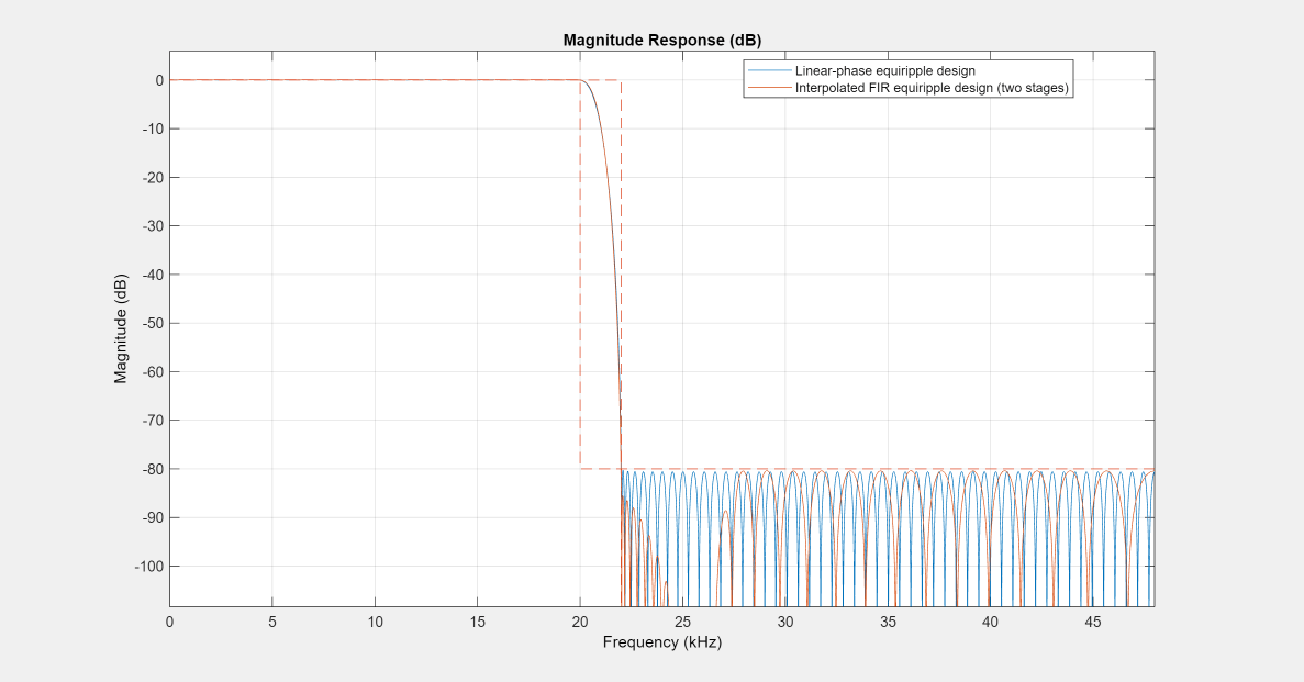
A different approach to minimizing the number of coefficients that does not involve minimum-phase designs is to use multistage techniques. This example showcases the interpolated FIR (IFIR) approach. This approach breaks down the design problem into designing two filters in a cascade. For this example, the design requires 151 coefficients rather than 173. For more information on multistage design techniques, see Efficient Narrow Transition-Band FIR Filter Design.
Design a filter using the Interpolated FIR (IFIR) design algorithm. Compute the cost of implementing the filter.
Fp  = 20e3;
Fst = 22e3;
Fs  = 96e3;
Ap  = 0.06;
Ast = 80;
interpFilter = designfilt("lowpassfir",PassbandFrequency=Fp,StopbandFrequency=Fst, ...
    PassbandRipple=Ap,StopbandAttenuation=Ast,SampleRate=Fs, ...
    DesignMethod="ifir",SystemObject=true);
cost(interpFilter)
ans = struct with fields:
                  NumCoefficients: 151
                        NumStates: 238
    MultiplicationsPerInputSample: 151
          AdditionsPerInputSample: 149
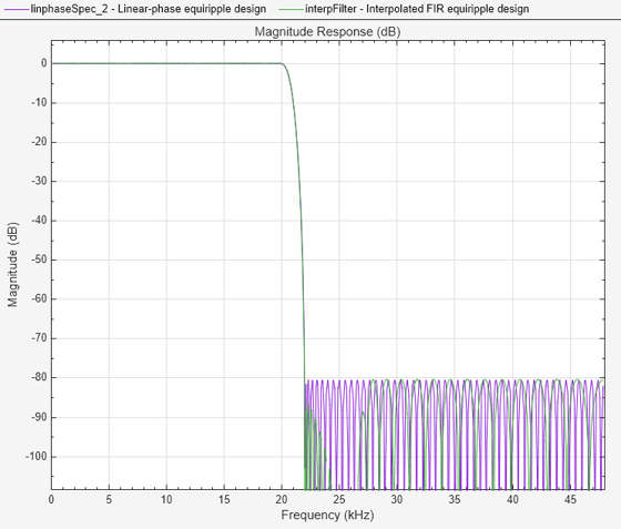
Compare the IFIR design with the linear-phase design using Filter Analyzer.
fvt = filterAnalyzer(linphaseSpec,interpFilter);
setLegendStrings(fvt,...
    ["Linear-phase equiripple design",...
    "Interpolated FIR equiripple design"]);
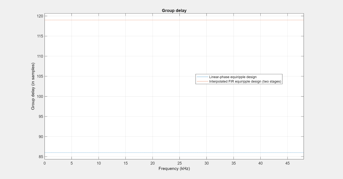
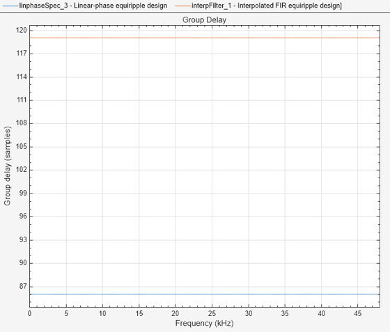
Plot the group delay of the IFIR design. While IFIR designs provide linear phase, their group delay is in general larger than that in a comparable single-stage design.
fvt = filterAnalyzer(linphaseSpec,interpFilter,Analysis='groupdelay');
setLegendStrings(fvt,...
    ["Linear-phase equiripple design",...
    "Interpolated FIR equiripple design]"])
Lowpass Filter Design for Multirate Applications
Lowpass filters are extensively used in the design of decimators and interpolators. For more information, see Design of Decimators and Interpolators. For more information on multistage techniques that result in very efficient implementations, see Multistage Rate Conversion.