Deploy Direction of Arrival Estimation Using Deep Learning on Raspberry Pi
This example shows how to generate and deploy code to estimate direction of arrival (DOA) using deep learning techniques on a Raspberry Pi with Simulink® in external mode simulation.
This example uses ARM NeonV7 CRL to generate optimized code for deployment.
Complete these examples to understand the fundamentals of direction of arrival estimation with deep learning:
Complete the steps in Build and Deploy Your First Simulink Model to Raspberry Pi (Raspberry Pi Blockset) to make sure that the Raspberry Pi device can run the steps outlined in this example.
Deep DOA Estimator Model
This example uses the same network trained in the Deploy Direction of Arrival Estimation Using Deep Learning on Desktop example for estimating DOA. Load the trained network.
if (exist("deepDOAEstimator.mat",'file') ~= 2)
    zipFile = matlab.internal.examples.downloadSupportFile("dsp","DeepDOAEstimator.zip");
    dataFolder = fileparts(zipFile);
    unzip(zipFile,cd)
end
file = load("deepDOAEstimator.mat");
deepDOAEstimator = file.deepDOAEstimator;
Simulink model
This example uses the same Simulink models created in the Deploy Direction of Arrival Estimation Using Deep Learning on Desktop example.
Open the referenced models that perform detection using deep learning and MUSIC algorithms.
topMdl = 'DOAEstimationTopModel';
open_system(topMdl)
refMdlDOA = 'DeepDOAEstimationModel';
open_system(refMdlDOA);
refMdlMUSIC = 'MusicDOAEstimationModel';
open_system(refMdlMUSIC);
You can configure the referenced model interactively by using the Configuration Parameters dialog box from the Simulink model toolstrip, or programmatically by using the MATLAB command-line interface.
Configure Model Using UI
To configure a referenced Simulink model to generate code, complete these steps for all three models DOAEstimationTopModel, MusicDOAEstimationModel, and DeepDOAEstimationModel.
Open the Simulink model. In the Modeling tab of the referenced model, click Model Settings to open the Configuration Parameters dialog box.
In the Hardware Implementation pane, set the Hardware board parameter to
Raspberry PiorRaspberry Pi (64 bit)based on your hardware device.In the Hardware board settings pane, expand Target hardware resources and select Board Parameters. Specify these parameter values:
Device Address: The IP address or host name of the hardware.
Username: Specify the root user name of the Linux® system running on the hardware. The default user name of the Raspian Linux distribution is
pi.Password: Specify the root password of the Linux system running on the hardware. The default password of the Raspian Linux distribution is
raspberry.
In the Code Generation pane:
Set System target file to
ert.tlc.Set Language to
C.Set Build configuration to
Faster Runsto prioritize execution speed.In the Verification pane, select Measure task execution time and set Measure function execution times to
Coarse (reference models and subsystems only).To generate optimized code, in the Optimization pane, set Leverage target hardware instruction set instructions to
Neon v7. Select Optimize reductions and FMA.
Under Code Generation, in the Code Style pane, set Dynamic array container type to
coder::array.In the Simulation Target pane, enable Dynamic memory allocation in MATLAB functions.
Configure Model Using Programmatic Approach
Alternatively, you can set all the configurations using set_param commands.
Set the Hardware board parameter to Raspberry Pi or Raspberry Pi (64 bit) based on your hardware device
set_param(refMdlDOA,'HardwareBoard','Raspberry Pi')
set_param(refMdlMUSIC,'HardwareBoard','Raspberry Pi')
set_param(topMdl,'HardwareBoard','Raspberry Pi')
Set the parameters for code generation.
set_param(refMdlDOA,'TargetLang','C')
set_param(refMdlDOA,'SystemTargetFile','ert.tlc')
set_param(refMdlDOA,'BuildConfiguration','Faster Runs')

set_param(topMdl,'TargetLang','C')
set_param(topMdl,'SystemTargetFile','ert.tlc')
set_param(topMdl,'BuildConfiguration','Faster Runs')

set_param(refMdlMUSIC,'TargetLang','C')
set_param(refMdlMUSIC,'SystemTargetFile','ert.tlc')
set_param(refMdlMUSIC,'BuildConfiguration','Faster Runs')
Enable dynamic memory allocation for MATLAB functions. Set the dynamic array container type to 'coder::array'. Enable code execution profiling.
set_param(refMdlDOA,'MATLABDynamicMemAlloc','on','DynamicArrayContainerType','coder::array',...
    'CodeExecutionProfiling','on')
set_param(topMdl,'MATLABDynamicMemAlloc','on','DynamicArrayContainerType','coder::array',...
    'CodeExecutionProfiling','on')
set_param(refMdlMUSIC,'MATLABDynamicMemAlloc','on','DynamicArrayContainerType','coder::array',...
    'CodeExecutionProfiling','on')
Enable ARM NeonV7 CRL optimization to generate optimized code.
set_param(refMdlDOA,'InstructionSetExtensions','Neon v7','OptimizeReductions','on',...
    'InstructionSetFMA','on')
set_param(topMdl,'InstructionSetExtensions','Neon v7','OptimizeReductions','on',...
    'InstructionSetFMA','on')
set_param(refMdlMUSIC,'InstructionSetExtensions','Neon v7','OptimizeReductions','on',...
    'InstructionSetFMA','on')
Save and close the referenced models.
close_system(refMdlDOA,1)
close_system(refMdlMUSIC,1)
In the top model, set the Simulation mode parameter of the model reference block to 'Normal'.
set_param([topMdl '/' refMdlDOA],'SimulationMode','Normal')
set_param([topMdl '/' refMdlMUSIC],'SimulationMode','Normal')
Run Simulink Model in External Mode
On the Hardware tab of the Simulink model, in the Mode section, select Run on board and then click Monitor & Tune.
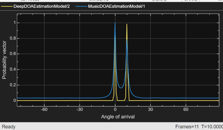
The Array Plot block shows the probability distribution of DOA estimation using deep learning, as well as the pseudospectrum from DOA estimation using MUSIC. The display blocks also displays the detected angles of arrival.
Profiling results
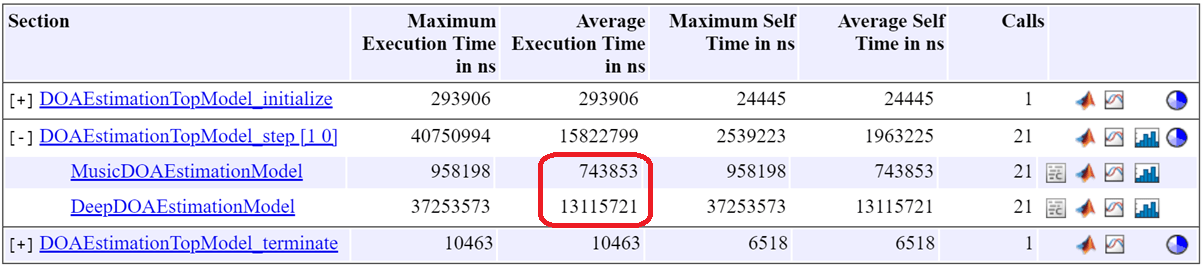
In this example, the average execution time for the step function in the deep DOA detector (13 ms) is higher than that of the MUSIC DOA detector (0.7 ms), as expected. However, both runtimes are sufficiently low to support reliable real‑time deployment.