Interpretable Time Series Forecasting Using a Temporal Fusion Transformer
This example shows how to forecast electricity usage using a temporal fusion transformer (TFT) [1]. TFT is an attention-based network that you can use for time series forecasting. The network uses attention mechanisms and importance weighting to provide interpretable insights into the importance of different time steps and features.
A TFT takes as input past values of a time series, along with other static and time-varying inputs, and outputs a prediction of future values for a specified number of time steps. The inputs to the TFT can be:
Known time-varying inputs — Inputs where the future values are known ahead of prediction time.
Unknown time-varying inputs — Inputs where the future values are not known ahead of prediction time. The response variable (the value you want to predict) is always an unknown input.
Static inputs — Inputs that do not change with time.
The inputs to the network can be numeric or categorical.
This example uses a TFT to forecast electricity usage of multiple clients at hourly intervals over one day, using the previous seven days' usage as input. The model also uses the following inputs:
Hour of day (known time-varying, numeric)
Day of week (known time-varying, numeric)
Hours since start of measurement (known time-varying, numeric)
Client ID (static, categorical).
For reproducibility, set the random seed.
rng(0)
Load and Visualize Data
This example uses a preprocessed version of the Electricity Load Diagrams data set available in the UCI Machine Learning Repository [2] and licensed under CC BY 4.0. The original data set contains values in kW of 370 clients, logged every 15 minutes from 2011 to 2014. The subset contains the hourly electricity consumption (in kWh) from January 1st 2014 to September 8th 2014, partitioned into training, validation, and test sets. Missing data is represented by NaN values. The data is approximately 10MB in size. Download the data from the MathWorks website.
filenameData = matlab.internal.examples.downloadSupportFile('nnet','data/ElectricityLoadDiagrams2014.mat')
load(filenameData)
Each data set contains a timetable. The rows represent the logged kWh. The columns represent the time and the 370 clients.
Plot the first 192 hours (eight days) of the sixth client in the training data set. The data shows a strong seasonal trend with a 24-hour period.
clientIdx = 6;
hrs = 1:192;
plot(tftUsageDataTrain.Time(hrs),tftUsageDataTrain{hrs,clientIdx});
xlabel("Time")
ylabel("Electricity Consumption (kWh)")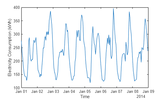
Extract the IDs of the electricity clients.
clientIDs = string(tftUsageDataTrain.Properties.VariableNames);
Prepare Data for Forecasting
Use the helper function addTimePredictorVariables to add extra columns to each table for hour of day, day of week, and number of hours since the start of the training time series.
startTime = tftUsageDataTrain.Properties.StartTime;

tftUsageDataTrain = addTimePredictorVariables(tftUsageDataTrain,startTime);
tftUsageDataValidation = addTimePredictorVariables(tftUsageDataValidation,startTime);
tftUsageDataTest = addTimePredictorVariables(tftUsageDataTest,startTime);
Normalize Data
Normalize the training data to have a mean of zero and a standard deviation of one. Normalize the validation and test data using the training data statistics. When computing the mean and standard deviation, use the "omitmissing" flag to ignore NaN values in the data.
trainingMean = mean(tftUsageDataTrain,"omitmissing");
trainingStd = std(tftUsageDataTrain,"omitmissing");

dataTrainNormalized = (tftUsageDataTrain - trainingMean) ./ trainingStd;
dataValidationNormalized = (tftUsageDataValidation - trainingMean) ./ trainingStd;
dataTestNormalized = (tftUsageDataTest - trainingMean) ./ trainingStd;
Chunk Data
Use the helper function chunkData to randomly sample the data into 192-hour (eight-day) chunks, which can overlap.
This example uses 45,000 samples for training, 5,000 samples for validation, and 5,000 samples for testing. To reproduce the results from [1], set numTrainSamples to 450,000, numValSamples to 50,000, and numTestSamples to "all".
sampleLength = 192;

numTrainSamples = 45000;
numValSamples = 5000;
numTestSamples = 5000;

[samplesTrain,idsTrain] = chunkData(dataTrainNormalized,sampleLength,numTrainSamples,clientIDs);
[samplesValidation,idsValidation] = chunkData(dataValidationNormalized,sampleLength,numValSamples,clientIDs);
[samplesTest,idsTest] = chunkData(dataTestNormalized,sampleLength,numTestSamples,clientIDs);
Create Datastore
Create datastores to store the multi-input data and process it for training the neural network using the createMultiInputDatastore helper function. Use 168 hours (7 days) of electricity load as input to the network and 24 hours (1 day) of electricity load as the target to forecast.
numPastTimeSteps = 168;
numFutureTimeSteps = 24;

dsTrain = createMultiInputDatastore(samplesTrain,numPastTimeSteps,idsTrain);
dsValidation = createMultiInputDatastore(samplesValidation,numPastTimeSteps,idsValidation);
dsTest = createMultiInputDatastore(samplesTest,numPastTimeSteps,idsTest);
Plot an example of the preprocessed training data.
[elecIn,hour,day,hoursFromStart,id,elecOut] = dsTrain.preview{:};

figure
tiledlayout(4,1)

nexttile
plot(1:numPastTimeSteps,elecIn)
hold on
plot(numPastTimeSteps+1:sampleLength,elecOut,'--')
hold off
legend(["Input" "Target"],Location="northwest")
ylabel("Electricity")

nexttile
plot(1:sampleLength,hour)
ylabel("Hour")

nexttile
plot(1:sampleLength,day)
ylabel("Day")

nexttile
plot(1:sampleLength,hoursFromStart)
ylabel("Hours from start")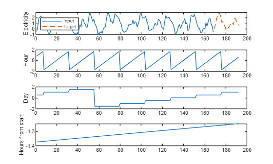
Create and Explore Temporal Fusion Transformer Network
Use the helper function createTFTNetwork to create the temporal fusion transformer network. To access this function, open the example as a live script.
Create a network with an architecture following [1]:
Specify one unknown, time-varying, continuous input (electricity).
Specify three known, time-varying, continuous inputs (hour, day, and hours from start).
Specify one static, categorical input (ID), with 370 categories.
Use 160 hidden units in each component.
Use four heads in the self-attention component.
Output predictions for three quantiles.
Use a dropout probability of 0.1.
inputNames = ["electricity" "hour" "day" "hoursFromStart" "id"];
unknownTimeVaryingInputIdx = 1;
knownTimeVaryingInputIdx = [2 3 4];
staticInputIdx = 5;
categoricalInputIdx = 5;
numCategories = 370;
numHiddenUnits = 160;
numAttentionHeads = 4;
numQuantiles = 3;
dropoutProbability = 0.1;

net = createTFTNetwork(inputNames,unknownTimeVaryingInputIdx, ...
    knownTimeVaryingInputIdx,staticInputIdx,categoricalInputIdx, ...
    numCategories,numHiddenUnits,numAttentionHeads,numPastTimeSteps, ...
    numFutureTimeSteps,numQuantiles, ...
    DropoutProbability=dropoutProbability);
Visualize Network
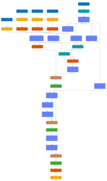
To view the network, use the Deep Network Designer app.
deepNetworkDesigner(net)
The network is made up of several different components contained in networkLayer objects. To view the contents of a network layer, double click the layer in Deep Network Designer.
Gated Linear Units
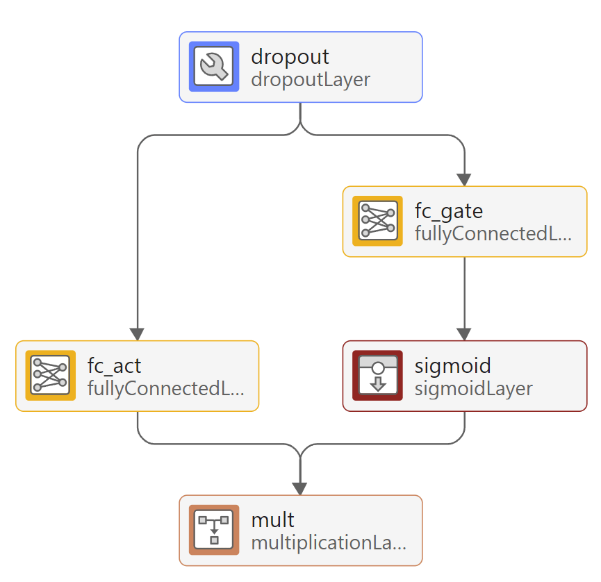
TFTs use gated linear unit (GLU) activations. To view an example of a GLU, double-click on the lstm_gate layer in Deep Network Designer.
A GLU is a learnable activation function that allows the network to control how much of the input to propagate through the network by returning high or low values from the sigmoid activation. To create a GLU network layer, use the gluNetworkLayer helper function included with this example.
Gated Residual Networks
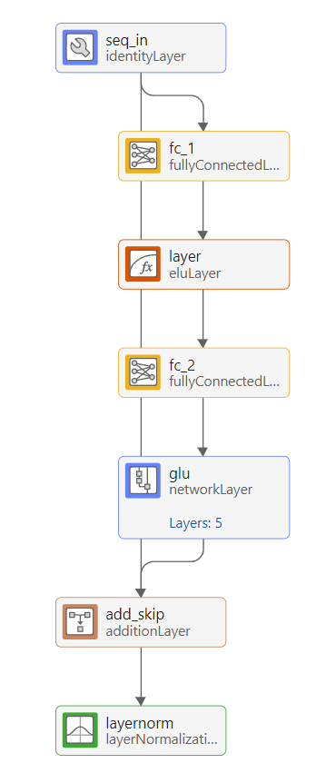
TFTs use gated residual networks (GRN) for nonlinear processing. These consist of fully connected layers with exponential linear unit (ELU) activations, and a gated skip connection using a GRU. To view an example of a GRN, double-click on the static_context_varselect layer in Deep Network Designer.
If the nonlinear processing is not helpful for the predictions of the network, then the GRU learns to suppress the nonlinear branch, effectively skipping the unit. To create a GRN network layer, use the grnNetworkLayer function included with this example.
Variable Selection Networks
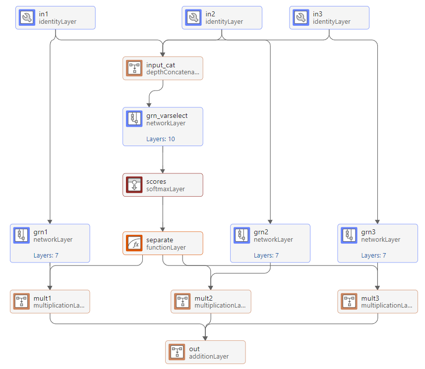
The known, unknown, and static data are inputs into the variable selection networks. A variable selection network aggregates the inputs with a learned weighting that depends on the input values. To view an example of a variable selection network, double-click on the layer future_varselect in Deep Network Designer. This layer performs variable selection on three input variables: the future values of the hour, day, and hoursFromStart inputs.
The variable selection network allows the TFT to amplify important inputs and suppress less important ones. You can interpret the outputs of the softmax layer as importance scores, allowing you to see which input features the network learns are most important for forecasting. To create a variable selection network layer, use the variableSelectionNetworkLayer function included with this example.
Interpretable Multi-Head Self-Attention
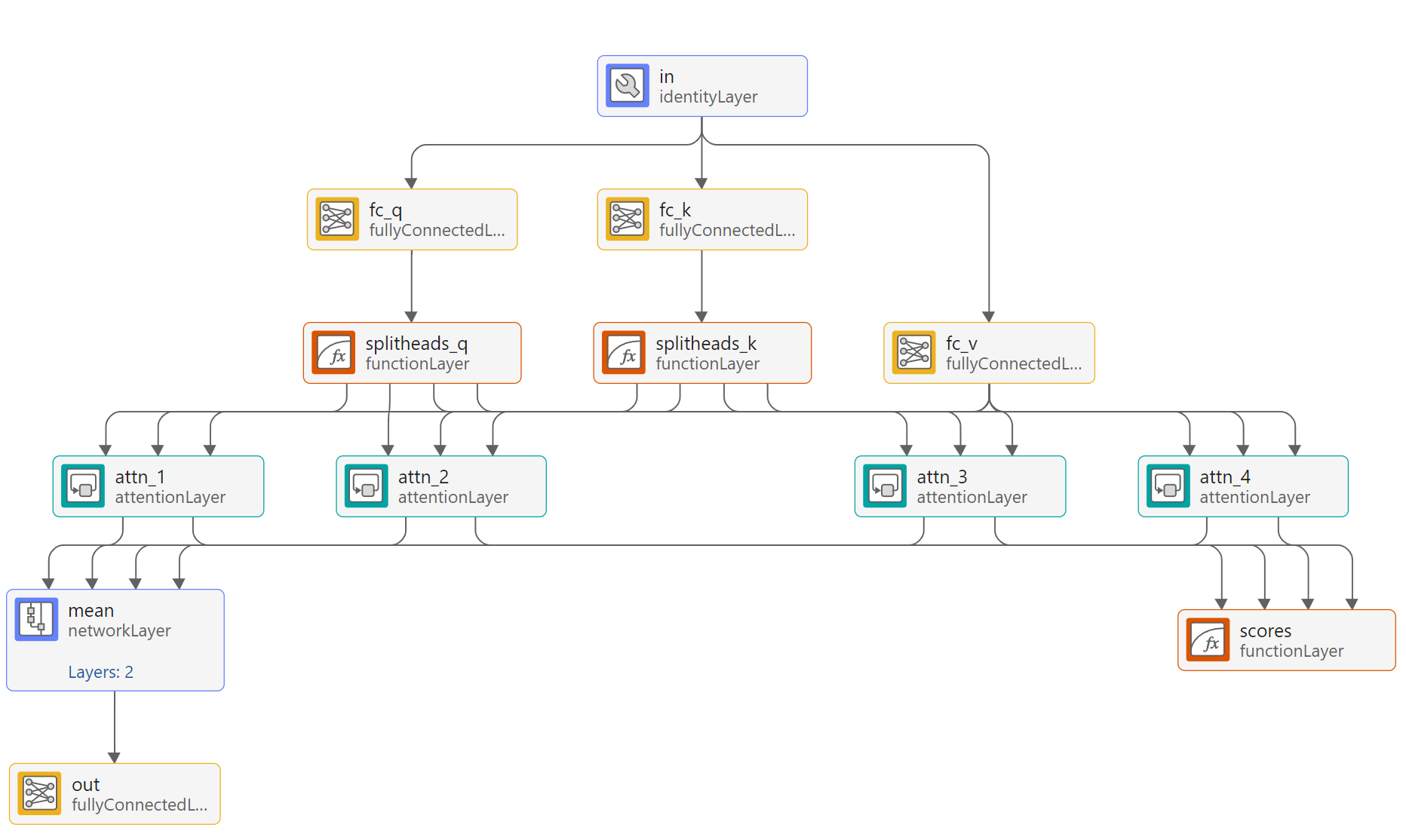
The TFT uses a variant of multi-head attention which, rather than concatenating, takes the average attention weights from each head and shares the values between attention heads. To view an example of an interpretable multi-head self-attention layer, double-click on the attn layer in Deep Network Designer. This layer has four attention heads.
You can interpret the attention scores from this layer because the network uses the same values for each head, meaning you can directly compare the scores from each head. To create an interpretable multi-head self-attention network layer, use the interpretableSelfAttentionNetworkLayer function included with this example.
Specify Training Options
Specify the training options.
Train using Adam optimization.
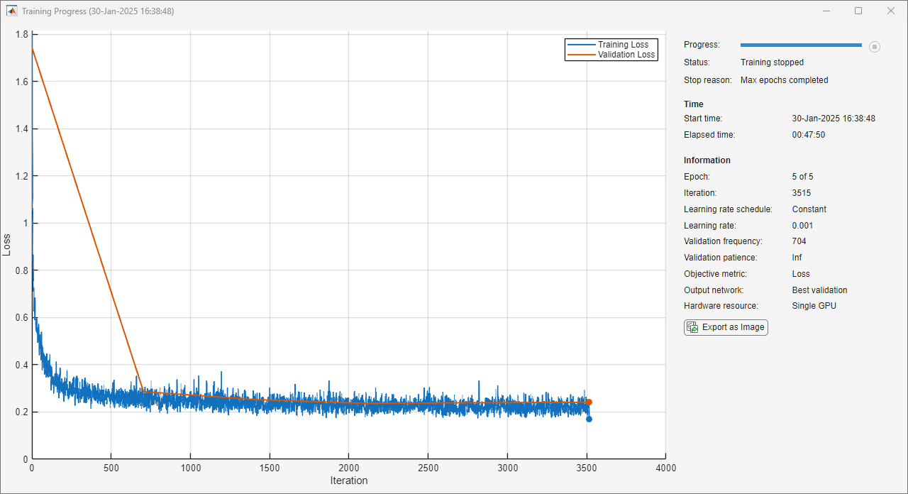
Train for 5 epochs.
Use a mini-batch size of 64.
Use an initial learning rate of 0.001.
Use a gradient threshold of 0.01.
Shuffle the data every epoch.
Use
dsValidationas validation data.Validate once per epoch.
Display the training progress in a plot.
Disable the verbose output.
minibatchsize = 64;
validationFrequency = ceil(numTrainSamples/minibatchsize);

options = trainingOptions("adam", ...
    MaxEpochs=5, ...
    MiniBatchSize=64, ...
    InitialLearnRate=0.001, ...
    GradientThreshold=0.01, ...
    Shuffle="every-epoch", ...
    ValidationData=dsValidation, ...
    ValidationFrequency=validationFrequency, ...
    Plots="training-progress", ...
    Verbose=false);
Train Temporal Fusion Transformer
Train the temporal fusion transformer network using the trainnet function. Use the custom loss function quantileLoss to train the network to predict the 10th, 50th, and 90th percentile forecasts. By default, the trainnet function uses a GPU if one is available. Using a GPU requires a Parallel Computing Toolbox™ license and a supported GPU device. For more information on supported devices, see GPU Computing Requirements (Parallel Computing Toolbox). Otherwise, the function uses the CPU. To specify the execution environment, use the ExecutionEnvironment training option.
Training the model is a computationally expensive process. To save time while running this example, set doTraining to false to load a pretrained network. The pretrained network is approximately 10MB in size. To train the network yourself, set doTraining to true.
quantiles = [0.1; 0.5; 0.9];

doTraining = false;
if doTraining
    trainedNet = trainnet(dsTrain,net,@(Y,T) quantileLoss(Y,T,quantiles,DataFormat="CBT"),options);
else
    fileNameNetwork = matlab.internal.examples.downloadSupportFile('nnet','data/ElectricityLoadForecastingTemporalFusionTransformer.mat');
    load(fileNameNetwork)
end
Test Network on Unseen Data
Use the minibatchpredict function to use the trained network to forecast electricity usage values on the test set. Use the Outputs name-value argument to also compute the variable selection importance scores from the network. Denormalize the predicted values using the training data statistics.
[testPredictions,testPastImportance,testFutureImportance] = minibatchpredict(trainedNet, ...
    dsTest, ...
    Outputs=["quantile_out","past_varselect/scores","future_varselect/scores"]);

denormalizedTestPredictions = denormalize(testPredictions,idsTest,trainingMean,trainingStd);
denormalizedTestTargets = denormalize(samplesTest(numPastTimeSteps+1:end,1,:),idsTest,trainingMean,trainingStd);
Compute the quantile loss and -risk values over the test set. -risk is similar to the quantile loss, but it is calculated for each quantile separately and normalizes after computing the loss, rather than computing the loss on the normalized data.
testLoss = quantileLoss(testPredictions,samplesTest(numPastTimeSteps+1:end,1,:),quantiles)
testLoss = single

0.2530
testQRisk = qRiskMetric(denormalizedTestPredictions,denormalizedTestTargets,quantiles)
testQRisk = 1×3 single row vector

    0.0312    0.0611    0.0346
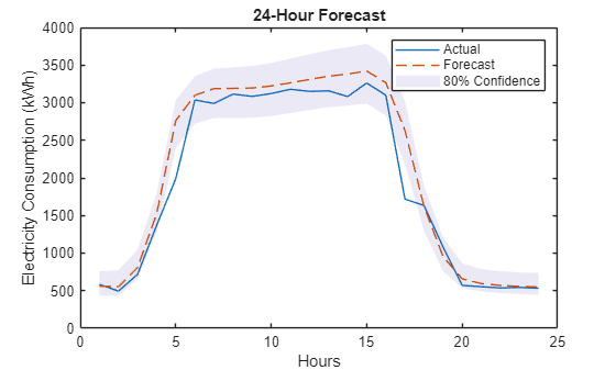
Compare the predictions with the targets. The three output channels in the prediction represent the 10th, 50th, and 90th percentile forecasts respectively. Plot the 50th percentile as the forecast and use the 10th and 90th as the bounds of the 80% confidence interval.
numTestSamples = size(samplesTest,3);
sampleIdx = randi(numTestSamples);
sampleToPlot = denormalizedTestTargets(:,:,sampleIdx);

figure
plot(sampleToPlot)
hold on
p10 = denormalizedTestPredictions(:,1,sampleIdx);
p50 = denormalizedTestPredictions(:,2,sampleIdx);
p90 = denormalizedTestPredictions(:,3,sampleIdx);
plot(p50, '--')
patch([1:numFutureTimeSteps flip(1:numFutureTimeSteps)]', ...
    [p10;flip(p90)],1, ...
    EdgeColor="none",FaceAlpha=0.1,CDataMapping="direct")

title("24-Hour Forecast")
xlabel("Hours")
ylabel("Electricity Consumption (kWh)")
legend(["Actual" "Forecast" "80% Confidence"])
hold off
Interpret Outputs of TFT Network
The TFT architecture allows you to analyze some of its individual components and interpret the relationships and patterns the model has learned.
Variable Importance
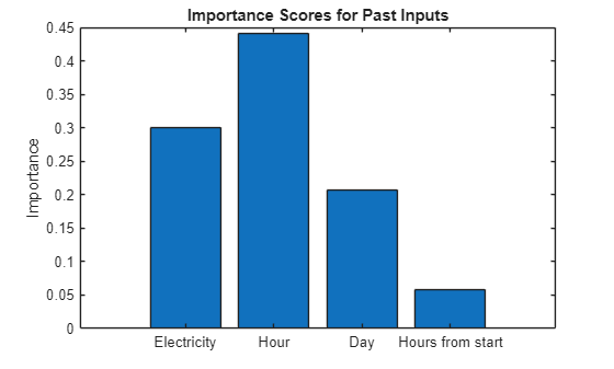
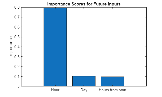
The output scores of the variable selection networks indicate the relative importance the network places on each input variable. Compute the median importance scores for the past and future inputs over all observations and time steps. The importance score for a variable is the weight that the network applies to the branch that processes that input variable. A higher importance score means the network gives a greater weight to that variable, implying it is more important to the predictions of the network.
observationDim = 3;
timeDim = 1;
medianPastImportance = median(testPastImportance,[observationDim timeDim]);
medianFutureImportance = median(testFutureImportance,[observationDim timeDim]);
Visualize the variable importance scores for past inputs. The scores show that hour of day and past electricity usage are the most important past input variables to the model.
figure
bar(medianPastImportance)
title("Importance Scores for Past Inputs")
ylabel("Importance")
xticklabels(["Electricity" "Hour" "Day" "Hours from start"]);
Visualize the variable importance scores for future inputs using a bar chart. The scores also show that hour of day is the most important future input variable to the model.
figure
bar(medianFutureImportance)
title("Importance Scores for Future Inputs")
ylabel("Importance")
xticklabels(["Hour" "Day" "Hours from start"]);
Attention Scores
You can use the scores output of the interpretable multi-head self-attention layer to analyze the most important past time steps the network uses in its prediction. Compute the attention scores for a subset of 1000 observations of the test data.
subsetSize = 1000;
sampleIdx = randsample(numTestSamples,subsetSize);
dsTestSubset = subset(dsTest,sampleIdx);

testAttnScores = minibatchpredict(trainedNet,dsTestSubset, ...
    Outputs="attn/scores",OutputDataFormats="UUUB");
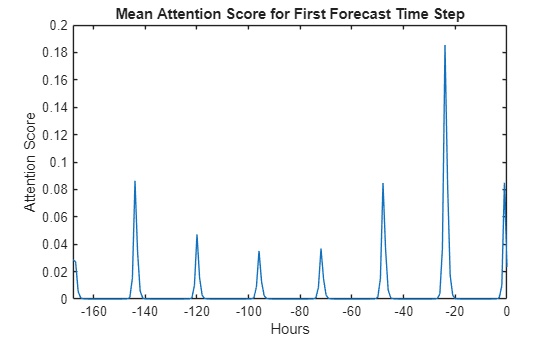
Compute the mean of the attention scores for the first future time step over all observations and attention heads.
headDim = 3;
observationDim = 4;
firstFutureTimeStep = numPastTimeSteps + 1;
meanAttentionScoreT1 = mean(testAttnScores(:,firstFutureTimeStep,:,:),[headDim observationDim]);
The causal masking in the attention layer means that the attention score between any time step and time steps in its future are zero. Remove the future time steps from the mean attention score.
meanAttentionScoreT1 = meanAttentionScoreT1(1:numPastTimeSteps+1);
Visualize the attention score across time steps. The attention scores show a peak every 24 hours, reflecting the strong 24-hour seasonal trend in the data.
figure
plot(-numPastTimeSteps:0,meanAttentionScoreT1)
title("Mean Attention Score for First Forecast Time Step")
xlabel("Hours")
ylabel("Attention Score")
xlim([-numPastTimeSteps 0])
References
Lim, Bryan, et al. “Temporal Fusion Transformers for Interpretable Multi-Horizon Time Series Forecasting.” International Journal of Forecasting, vol. 37, no. 4, Oct. 2021, pp. 1748–64. ScienceDirect, https://doi.org/10.1016/j.ijforecast.2021.03.012.
Trindade, A. (2015). ElectricityLoadDiagrams20112014 [Dataset]. UCI Machine Learning Repository. https://doi.org/10.24432/C58C86
Wen, Ruofeng, et al. A Multi-Horizon Quantile Recurrent Forecaster. arXiv:1711.11053, arXiv, 28 June 2018. arXiv.org, https://doi.org/10.48550/arXiv.1711.11053.
Supporting Functions
Predictor Creation Function
The function addTimePredictorVariables computes extra time variables and adds them to the table. The time variables are hour of day, day of week, and hours since the start time.
function tbl = addTimePredictorVariables(tbl,startTime)
tbl.Hour = hour(tbl.Time);
tbl.Day = day(tbl.Time, "dayofweek");
tbl.HoursFromStart = hours(tbl.Time - startTime);
end
Data Chunking Function
The function chunkData randomly chooses numSamples samples of length chunkLength from the input data. To chunk the entire input data, set numSamples to "all".
function [samples,ids] = chunkData(data,chunkLength,numSamples,allIDs)
% Compute all valid sample points in the form (row, column)
validSampleLocations = [];
numIDs = numel(allIDs);

for ii = 1:numIDs
    % Ignore leading and trailing NaNs
    startIdx = find(~ismissing(data.(allIDs(ii))),1);
    endIdx = find(~ismissing(data.(allIDs(ii))),1,"last");
    numValidTimeSteps = endIdx - startIdx + 1;

    if numValidTimeSteps > chunkLength
        numSamplesPerObservation = numValidTimeSteps - chunkLength + 1;
        locs = [(startIdx:startIdx+numSamplesPerObservation-1)',ii*ones(numSamplesPerObservation,1)];
        validSampleLocations = [validSampleLocations;locs];
    end
end

% Randomly choose sample points without replacement
if strcmp(numSamples,"all")
    numSamples = size(validSampleLocations,1);
    locsToChoose = 1:size(validSampleLocations,1);
else
    locsToChoose = randsample(size(validSampleLocations,1),numSamples);
end

numFeatures = 4; % Electricity, hour, day, hours from start
samples = zeros(chunkLength,numFeatures,numSamples);
ids = categorical(strings(numSamples,1),allIDs);

% Sample
for ii = 1:numSamples
    startRow = validSampleLocations(locsToChoose(ii),1);
    id = allIDs(validSampleLocations(locsToChoose(ii),2));

    samples(:,1,ii) = data.(id)(startRow:startRow+chunkLength-1);
    samples(:,2,ii) = data.Hour(startRow:startRow+chunkLength-1);
    samples(:,3,ii) = data.Day(startRow:startRow+chunkLength-1);
    samples(:,4,ii) = data.HoursFromStart(startRow:startRow+chunkLength-1);

    ids(ii) = id;
end
end
Datastore Creation Function
The function createMultiInputDatastore prepares the inputs and outputs for neural network training by creating a datastore.
function ds = createMultiInputDatastore(samples,numPastTimeSteps,ids)
adsElecInputs = arrayDatastore(samples(1:numPastTimeSteps,1,:),IterationDimension=3);
adsElecTargets = arrayDatastore(samples(numPastTimeSteps+1:end,1,:),IterationDimension=3);
adsHour = arrayDatastore(samples(:,2,:),IterationDimension=3);
adsDay = arrayDatastore(samples(:,3,:),IterationDimension=3);
adsHoursFromStart = arrayDatastore(samples(:,4,:),IterationDimension=3);
adsID = arrayDatastore(ids);

ds = combine(adsElecInputs,adsHour,adsDay,adsHoursFromStart,adsID,adsElecTargets);
end
Quantile Loss Function
The quantileLoss function computes the quantile loss [3] for the specified quantiles, summed over all quantile outputs:
where the quantile loss
Here a target time series to forecast, is the model's prediction, is the total number of observations, is the total number of forecast time steps, is the quantile being forecast, and is the set of all quantiles (in this example ). If , then the quantile loss encourages the model to underpredict the true value. If , then the quantile loss encourages the model to overpredict. When the quantile loss is the same as the L1 loss (mean absolute error).
function l = quantileLoss(Y,T,quantiles,options)
arguments
    Y
    T
    quantiles
    options.DataFormat = "TCB"
end

predictionUnderflow = T - Y;
channelDim = strfind(options.DataFormat,"C");
quantiles = shiftdim(quantiles,1-channelDim);

qLoss = quantiles .* max(predictionUnderflow,0) + (1 - quantiles) .* max(-predictionUnderflow,0);

observationDim = strfind(options.DataFormat,"B");
timeDim = strfind(options.DataFormat,"T");
numObservations = size(Y,observationDim);
numTimeSteps = size(Y,timeDim);
l = sum(qLoss,"all") / (numObservations*numTimeSteps);
end
q-risk Metric Function
The qRiskMetric function computes the -risk for the specified quantiles:
.
You can use the -risk to compare the results to Ref. [1] and the other papers it references. The results in this example do not match the results in Ref. [1] because this example trains on a smaller subset of the ElectricityLoadDiagrams20112014 data set.
function qRisk = qRiskMetric(Y,T,quantiles)
predictionUnderflow = T - Y;
weightedErrors = quantiles' .* max(predictionUnderflow,0) + (1 - quantiles') .* max(-predictionUnderflow,0);

quantileLoss = mean(weightedErrors, [1 3]);
normalizer = mean(abs(T), [1 3]);

qRisk = 2*quantileLoss/normalizer;
end
Denormalization Function
The denormalize function denormalizes the predictions made by the TFT.
function denormalizedPredictions = denormalize(predictions,ids,trainingMean,trainingStd)
mu = shiftdim(trainingMean{:,double(ids)},-1);
sigma = shiftdim(trainingStd{:,double(ids)},-1);

denormalizedPredictions = predictions .* sigma + mu;
end
See Also
dlnetwork | trainnet | attentionLayer | Deep Network
Designer | networkLayer