Design Neural Network Predictive Controller in Simulink
The neural network predictive controller that is implemented in the Deep Learning Toolbox™ software uses a neural network model of a nonlinear plant to predict future plant performance. The controller then calculates the control input that will optimize plant performance over a specified future time horizon. The first step in model predictive control is to determine the neural network plant model (system identification). Next, the plant model is used by the controller to predict future performance. (See the Model Predictive Control Toolbox™ documentation for complete coverage of the application of various model predictive control strategies to linear systems.)
The following section describes the system identification process. This is followed by a description of the optimization process. Finally, it discusses how to use the model predictive controller block that is implemented in the Simulink® environment.
Note
To design a neural network predictive controller, you can also use System Identification Toolbox™ and Model Predictive Control Toolbox. Use System Identification Toolbox for plant modeling using a neural network and Model Predictive Control Toolbox to design the controller.
This workflow is recommended because of these advantages:
Decouple the plant modeling and control design.
Easy integration with Simulink using dedicated Simulink blocks for neural network plants and controllers.
Several built-in solvers for linear and nonlinear predictive control.
Supports code generation.
For an example showing how to use these tools, see Control House Heating Using Nonlinear MPC with Neural State-Space Prediction Model (Model Predictive Control Toolbox).
System Identification
The first stage of model predictive control is to train a neural network to represent the forward dynamics of the plant. The prediction error between the plant output and the neural network output is used as the neural network training signal. The process is represented by the following figure:
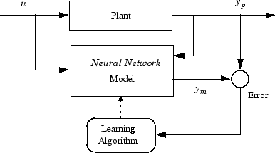
The neural network plant model uses previous inputs and previous plant outputs to predict future values of the plant output. The structure of the neural network plant model is given in the following figure.
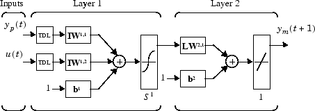
This network can be trained offline in batch mode, using data collected from the operation of the plant. You can use any of the training algorithms discussed in Multilayer Shallow Neural Networks and Backpropagation Training for network training. This process is discussed in more detail in following sections.
Predictive Control
The model predictive control method is based on the receding horizon technique [SoHa96]. The neural network model predicts the plant response over a specified time horizon. The predictions are used by a numerical optimization program to determine the control signal that minimizes the following performance criterion over the specified horizon
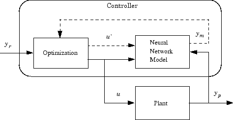
where N1, N2, and Nu define the horizons over which the tracking error and the control increments are evaluated. The u′ variable is the tentative control signal, yr is the desired response, and ym is the network model response. The ρ value determines the contribution that the sum of the squares of the control increments has on the performance index.
The following block diagram illustrates the model predictive control process. The controller consists of the neural network plant model and the optimization block. The optimization block determines the values of u′ that minimize J, and then the optimal u is input to the plant. The controller block is implemented in Simulink, as described in the following section.
Use the Neural Network Predictive Controller Block
This section shows how the NN Predictive Controller block is used. The first step is to copy the NN Predictive Controller block from the Deep Learning Toolbox block library to the Simulink Editor. See the Simulink documentation if you are not sure how to do this. This step is skipped in the following example.
An example model is provided with the Deep Learning Toolbox software to show the use of the predictive controller. This example uses a catalytic Continuous Stirred Tank Reactor (CSTR). A diagram of the process is shown in the following figure.
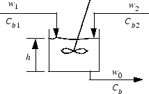
The dynamic model of the system is
where h(t) is the liquid level, Cb(t) is the product concentration at the output of the process, w1(t) is the flow rate of the concentrated feed Cb1, and w2(t) is the flow rate of the diluted feed Cb2. The input concentrations are set to Cb1 = 24.9 and Cb2 = 0.1. The constants associated with the rate of consumption are k1 = 1 and k2 = 1.
The objective of the controller is to maintain the product concentration by adjusting the flow w1(t). To simplify the example, set w2(t) = 0.1. The level of the tank h(t) is not controlled for this experiment.
To run this example:
Start MATLAB®.
Type
predcstrin the MATLAB Command Window. This command opens the Simulink Editor with the following model.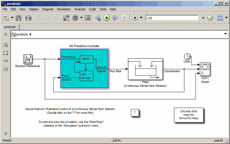
The Plant block contains the Simulink CSTR plant model. The NN Predictive Controller block signals are connected as follows:
Control Signal is connected to the input of the Plant model.
The Plant Output signal is connected to the Plant block output.
The Reference is connected to the Random Reference signal.
Double-click the NN Predictive Controller block. This opens the following window for designing the model predictive controller. This window enables you to change the controller horizons N2 and Nu. (N1 is fixed at 1.) The weighting parameter ρ, described earlier, is also defined in this window. The parameter α is used to control the optimization. It determines how much reduction in performance is required for a successful optimization step. You can select which linear minimization routine is used by the optimization algorithm, and you can decide how many iterations of the optimization algorithm are performed at each sample time. The linear minimization routines are slight modifications of those discussed in Multilayer Shallow Neural Networks and Backpropagation Training.
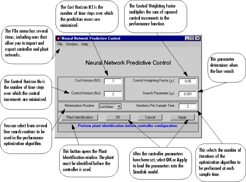
Select Plant Identification. This opens the following window. You must develop the neural network plant model before you can use the controller. The plant model predicts future plant outputs. The optimization algorithm uses these predictions to determine the control inputs that optimize future performance. The plant model neural network has one hidden layer, as shown earlier. You select the size of that layer, the number of delayed inputs and delayed outputs, and the training function in this window. You can select any of the training functions described in Multilayer Shallow Neural Networks and Backpropagation Training to train the neural network plant model.

Click Generate Training Data. The program generates training data by applying a series of random step inputs to the Simulink plant model. The potential training data is then displayed in a figure similar to the following.
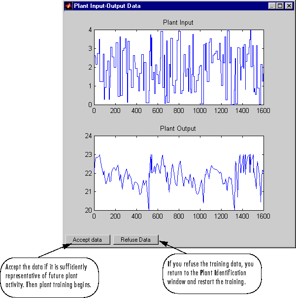
Click Accept Data, and then click Train Network in the Plant Identification window. Plant model training begins. The training proceeds according to the training algorithm (
trainlmin this case) you selected. This is a straightforward application of batch training, as described in Multilayer Shallow Neural Networks and Backpropagation Training. After the training is complete, the response of the resulting plant model is displayed, as in the following figure. (There are also separate plots for validation and testing data, if they exist.)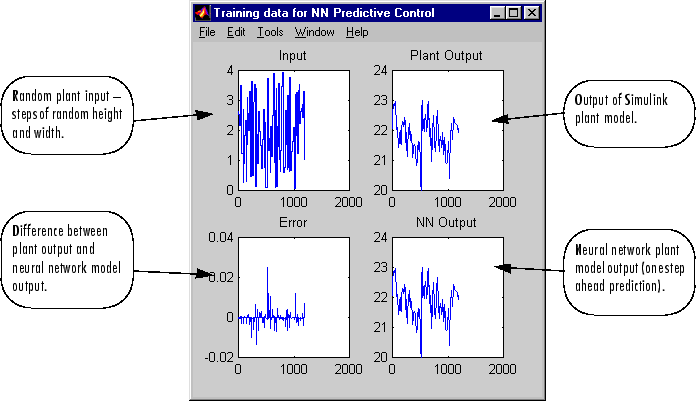
You can then continue training with the same data set by selecting Train Network again, you can Erase Generated Data and generate a new data set, or you can accept the current plant model and begin simulating the closed loop system. For this example, begin the simulation, as shown in the following steps.
Select OK in the Plant Identification window. This loads the trained neural network plant model into the NN Predictive Controller block.
Select OK in the Neural Network Predictive Control window. This loads the controller parameters into the NN Predictive Controller block.
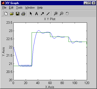
Return to the Simulink Editor and start the simulation by choosing the menu option Simulation > Run. As the simulation runs, the plant output and the reference signal are displayed, as in the following figure.
