Parameterize Gain Schedules
Typically, gain-scheduled control systems in Simulink® use lookup tables or MATLAB Function blocks to specify gain values as a function of the scheduling variables. For tuning, you replace these blocks by parametric gain surfaces. A parametric gain surface is a basis-function expansion whose coefficients are tunable. For example, you can model a time-varying gain k(t) as a cubic polynomial in t:
k(t) = k0 + k1t + k2t2 + k3t3.
Here,
k0,...,k3
are tunable coefficients. When you parameterize scheduled gains in this way,
systune can tune the gain-surface coefficients to meet your control
objectives at a representative set of operating conditions. For applications where gains vary
smoothly with the scheduling variables, this approach provides explicit formulas for the
gains, which the software can write directly to MATLAB Function blocks. When
you use lookup tables, this approach lets you tune a few coefficients rather than many
individual lookup-table entries, drastically reducing the number of parameters and ensuring
smooth transitions between operating points.
Basis Function Parameterization
In a gain-scheduled controller, the scheduled gains are functions of the scheduling variables, σ. For example, a gain-scheduled PI controller has the form:
Tuning this controller requires determining the functional forms Kp(σ) and Ki(σ) that yield the best system performance over the operating range of σ values. However, tuning arbitrary functions is difficult. Therefore, it is necessary either to consider the function values at only a finite set of points, or restrict the generality of the functions themselves.
In the first approach, you choose a collection of design points, σ, and tune the gains Kp and Ki independently at each design point. The resulting set of gain values is stored in a lookup table driven by the scheduling variables, σ. A drawback of this approach is that tuning might yield substantially different values for neighboring design points, causing undesirable jumps when transitioning from one operating point to another.
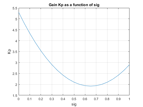
Alternatively, you can model the gains as smooth functions of σ, but restrict the generality of such functions by using specific basis function expansions. For example, suppose σ is a scalar variable. You can model Kp(σ) as a quadratic function of σ:
After tuning, this parametric gain might have a profile such as the following (the specific shape of the curve depends on the tuned coefficient values and range of σ):
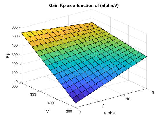
Or, suppose that σ consists of two scheduling variables, α and V. Then, you can model Kp(σ) as a bilinear function of α and V:
After tuning, this parametric gain might have a profile such as the following. Here too, the specific shape of the curve depends on the tuned coefficient values and ranges of σ values:
For tuning gain schedules with systune, you use a
parametric gain surface that is a particular expansion of the gain
in basis functions of σ:
The basis functions F1,...,FM are user-selected and fixed. These functions operate on n(σ), where n is a function that scales and normalizes the scheduling variables to the interval [–1,1] (or an interval you specify). The coefficients of the expansion, K0,...,KM, are the tunable parameters of the gain surface. K0,...,KM can be scalar or matrix-valued, depending on the I/O size of the gain K(σ). The choice of basis function is problem-dependent, but in general, try low-order polynomial expansions first.
Tunable Gain Surfaces
Use the tunableSurface command to construct a
tunable model of a gain surface sampled over a grid of design points (σ
values). For example, consider the gain with bilinear dependence on two scheduling
variables, α and V:
Suppose that α is an angle of incidence that ranges from 0° to 15°, and V is a speed that ranges from 300 m/s to 700 m/s. Create a grid of design points that span these ranges. These design points must match the parameter values at which you sample your varying or nonlinear plant. (See Plant Models for Gain-Scheduled Controller Tuning.)
[alpha,V] = ndgrid(0:5:15,300:100:700);
domain = struct('alpha',alpha,'V',V);
Specify the basis functions for the parameterization of this surface,
α, V, and αV. The
tunableSurface command expects the basis functions to be arranged as
a vector of functions of two input variables. You can use an anonymous function to express
the basis functions.
shapefcn = @(alpha,V)[alpha,V,alpha*V];
Alternatively, use polyBasis, fourierBasis, or ndBasis to generate basis functions of as
many scheduling variables as you need.
Create the tunable surface using the design points and basis functions.
Kp = tunableSurface('Kp',1,domain,shapefcn);Kp is a tunable model of the gain surface.
tunableSurface parameterizes the surface as:
where
The surface is expressed in terms of the normalized variables, rather than in terms of α and V.
This normalization, which tunableSurface performs by default, improves
the conditioning of the optimization performed by systune. If needed,
you can change the default scaling and normalization. (See tunableSurface).
The second input argument to tunableSurface specifies the initial
value of the constant coefficient, K0. By default,
K0 is the gain when all the scheduling variables
are at the center of their ranges. tunableSurface takes the I/O
dimensions of the gain surface from K0. Therefore,
you can create array-valued tunable gains by providing an array for that input.
Karr = tunableSurface('Karr',ones(2),domain,shapefcn);Karr is a 2-by-2 matrix in which each entry is a bilinear function of
the scheduling variables with independent coefficients.
Tunable Gain with Two Independent Scheduling Variables
This example shows how to model a scalar gain K with a bilinear dependence on two scheduling variables. You do so by creating a grid of design points representing the independent dependence of the two variables.
Suppose that the first variable α is an angle of incidence that ranges from 0 to 15 degrees, and the second variable V is a speed that ranges from 300 to 600 m/s. By default, the normalized variables are:
The gain surface is modeled as:
where are the tunable parameters.
Create a grid of design points, (α,V), that are linearly spaced in α and V. These design points are the scheduling-variable values used for tuning the gain-surface coefficients. They must correspond to parameter values at which you have sampled the plant.
[alpha,V] = ndgrid(0:3:15,300:50:600);
These arrays, alpha and V, represent the independent variation of the two scheduling variables, each across its full range. Put them into a structure to define the design points for the tunable surface.
domain = struct('alpha',alpha,'V',V);
Create the basis functions that describe the bilinear expansion.
shapefcn = @(x,y) [x,y,x*y]; % or use polyBasis('canonical',1,2)In the array returned by shapefcn, the basis functions are:
Create the tunable gain surface.
K = tunableSurface('K',1,domain,shapefcn);You can use the tunable surface as the parameterization for a lookup table block or a MATLAB Function block in a Simulink model. Or, use model interconnection commands to incorporate it as a tunable element in a control system modeled in MATLAB. After you tune the coefficients, you can examine the resulting gain surface using the viewSurf command. For this example, instead of tuning, manually set the coefficients to non-zero values and view the resulting gain.
Ktuned = setData(K,[100,28,40,10]);
viewSurf(Ktuned)
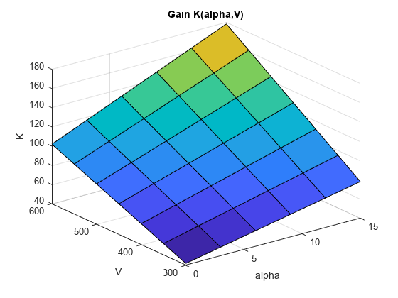
viewSurf displays the gain surface as a function of the scheduling variables, for the ranges of values specified by domain and stored in the SamplingGrid property of the gain surface.
Tunable Surfaces in Simulink
In your Simulink model, you model gain schedules using lookup table blocks, MATLAB
Function blocks, or Matrix Interpolation blocks, as described in
Model Gain-Scheduled Control Systems in Simulink. To tune these
gain surfaces, use tunableSurface to create a gain surface for each
block. In the slTuner interface to the model, designate each gain
schedule as a block to tune, and set its parameterization to the corresponding gain surface.
For instance, the rct_CSTR model includes a gain-scheduled PI controller,
the Concentration controller subsystem, in which the gains
Kp and Ki vary with the scheduling variable
Cr.
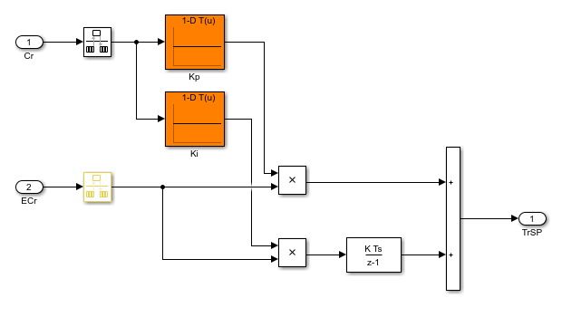
To tune the lookup tables Kp and Ki, create a
tunable surface for each one. Suppose that CrEQ is the vector of design
points, and that you expect the gains to vary quadratically with
Cr.
TuningGrid = struct('Cr',CrEQ);
ShapeFcn = @(Cr) [Cr , Cr^2];

Kp = tunableSurface('Kp',0,TuningGrid,ShapeFcn);
Ki = tunableSurface('Ki',-2,TuningGrid,ShapeFcn);
Suppose that you have an array Gd of linearizations of the plant
subsystem, CSTR, at each of the design points in CrEQ. (See
Plant Models for Gain-Scheduled Controller Tuning). Create an
slTuner interface that substitutes this array for the plant subsystem
and designates the two lookup-table blocks for tuning.
BlockSubs = struct('Name','rct_CSTR/CSTR','Value',Gd);
ST0 = slTuner('rct_CSTR',{'Kp','Ki'},BlockSubs);
Finally, use the tunable surfaces to parameterize the lookup tables.
ST0.setBlockParam('Kp',Kp);
ST0.setBlockParam('Ki',Ki);
When you tune STO, systune tunes the
coefficients of the tunable surfaces Kp and Ki, so
that each tunable surface represents the tuned relationship between Cr
and the gain. When you write the tuned values back to the block for validation,
setBlockParam automatically generates tuned lookup-table data by
evaluating the tunable surfaces at the breakpoints you specify in the corresponding blocks.
For more details about this example, see Gain-Scheduled Control of a Chemical Reactor.
Tunable Surfaces in MATLAB
For a control system modeled in MATLAB®, use tunable surfaces to construct more complex gain-scheduled control
elements, such as gain-scheduled PID controllers, filters, or state-space controllers. For
example, suppose that you create two gain surfaces Kp and
Ki using tunableSurface. The following command
constructs a tunable gain-scheduled PI controller.
C0 = pid(Kp,Ki);
Similarly, suppose that you create four matrix-valued gain surfaces
A, B, C, D. The
following command constructs a tunable gain-scheduled state-space controller.
C1 = ss(A,B,C,D);
You then incorporate the gain-scheduled controller into a generalized model of your
entire control system. For example, suppose G is an array of models of
your plant sampled at the design points that are specified in Kp and
Ki. Then, the following command builds a tunable model of a
gain-scheduled single-loop PID control system.
T0 = feedback(G*C0,1);
When you interconnect a tunable surface with other LTI models, the resulting model is an
array of tunable generalized genss models. The design points in the
tunable surface determine the dimensions of the array. Thus, each entry in the array
represents the system at the corresponding scheduling variable value. The
SamplingGrid property of the array stores those design points.
T0 = feedback(G*Kp,1)
T0 =

  4x5 array of generalized continuous-time state-space models.
  Each model has 1 outputs, 1 inputs, 3 states, and the following blocks:
    Kp: Parametric 1x4 matrix, 1 occurrences.

Type "ss(T0)" to see the current value, "get(T0)" to see all properties, and
"T0.Blocks" to interact with the blocks.
The resulting generalized model has tunable blocks corresponding to the gain surfaces
used to create the model. In this example, the system has one gain surface,
Kp, which has the four tunable coefficients corresponding to
K0,
K1, K2,
and K3. Therefore, the tunable block is a
vector-valued realp parameter with four entries.
When you tune the control system with systune, the software tunes
the coefficients for each of the design points specified in the tunable surface.
For an example illustrating the entire workflow in MATLAB, see the section "Controller Tuning in MATLAB" in Gain-Scheduled Control of a Chemical Reactor.