Frequency-Limited Balanced Truncation
This example shows how to reduce a high-order model by removing states of relatively low energy within a particular frequency interval. Focusing the energy-contribution calculation on a particular frequency region sometimes yields a good approximation to the dynamics of interest at a lower order than a reduction that takes all frequencies into account.
This example demonstrates frequency-limited balanced truncation at the command line, using options for the balanced truncation at the command line.
Load a model and examine its frequency response.
load('building.mat','G')
bodeplot(G)
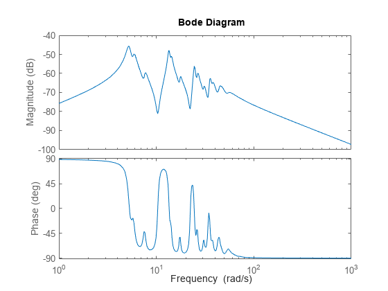
G is a 48th-order model with several large peak regions around 5.2 rad/s, 13.5 rad/s, and 24.5 rad/s, and smaller peaks scattered across many frequencies. Examine the Hankel singular-value plot to see the energy contributions of the model's 48 states.
R = reducespec(G,"balanced");
view(R)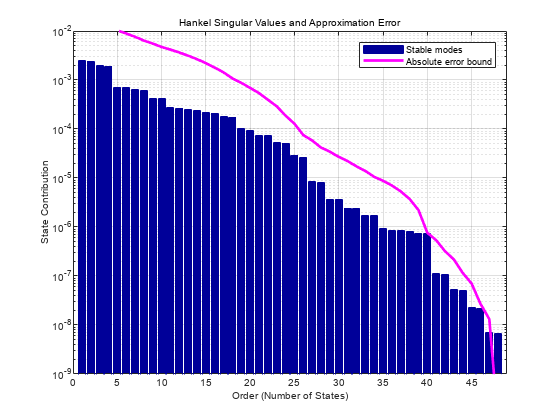
The singular-value plot suggests that you can discard at least 20 states without significant impact on the overall system response. Suppose that for your application you are only interested in the dynamics near the second large peak, between 10 rad/s and 22 rad/s. Try a few reduced-model orders based on the Hankel singular value plot. Compare their frequency responses to the original model, especially in the region of that peak.
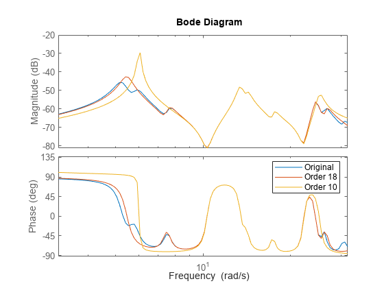
G18 = getrom(R,Order=18);
G10 = getrom(R,Order=10);

bodeplot(G,G18,G10,logspace(0.5,1.5,100));
legend('Original','Order 18','Order 10');
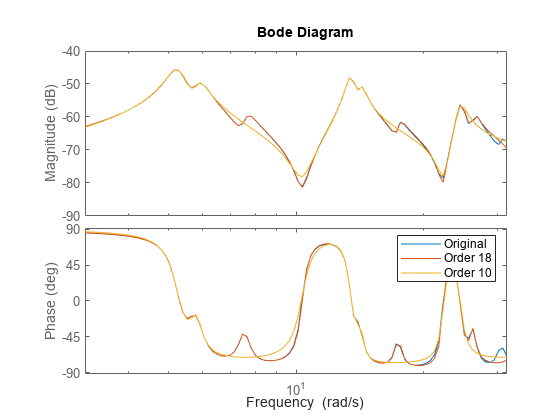
The 18th-order model is a good match to the dynamics in the region of interest. In the 10th order model, however, there is some degradation of the match.
Focus the model reduction on the region of interest to obtain a good match with a lower-order approximation. First, examine the state energy contributions in that frequency region only. Use R.Options.FreqIntervals to specify the frequency interval.
R.Options.FreqIntervals = [10,22];
view(R)
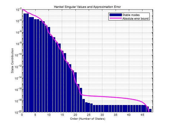
Comparing this plot to the previous Hankel singular-value plot shows that in this frequency region, many fewer states contribute significantly to the dynamics than contribute to the overall dynamics. Try the same reduced-model orders again, this time choosing states to eliminate based only on their contribution to the frequency interval.
GLim18 = getrom(R,Order=18,Method="Truncate");
GLim10 = getrom(R,Order=10,Method="Truncate");

bodeplot(G,GLim18,GLim10,logspace(0.5,1.5,100));
legend('Original','Order 18','Order 10');
With the frequency-limited energy computation, a 10th-order approximation is as good in the region of interest as the 18th-order approximation computed without frequency limits.