Main Content

passiveplot

Compute or plot passivity index as function of frequency

Description

example

passiveplot(G) plots the relative passivity indices of the dynamic system G as a function of frequency. When I + G is minimum phase, the relative passivity indices are the singular values of (I - G)(I + G)^-1. The largest singular value measures the relative excess (R < 1) or shortage (R > 1) at each frequency. See getPassiveIndex for more information about the meaning of the passivity index.

passiveplot automatically chooses the frequency range and number of points for the plot based on the dynamics of G.

If G is a model with complex coefficients, then in:

  • Log frequency scale, the plot shows two branches, one for positive frequencies and one for negative frequencies. The arrows indicate the direction of increasing frequency values for each branch.

  • Linear frequency scale, the plot shows a single branch with a symmetric frequency range centered at a frequency value of zero.

example

passiveplot(G,type) plots the input, output, or I/O passivity index, depending on the value of type: 'input', 'output', or 'io', respectively.

passiveplot(___,w) plots the passivity index for frequencies specified by w.

  • If w is a cell array of the form {wmin,wmax}, then passiveplot plots the passivity index at frequencies ranging between wmin and wmax.

  • If w is a vector of frequencies, then passiveplot plots the passivity index at each specified frequency. The vector w can contain both negative and positive frequencies.

You can use this syntax with any of the previous input-argument combinations.

passiveplot(G1,G2,...,GN,___) plots the passivity index for multiple dynamic systems G1,G2,...,GN on the same plot. You can also use this syntax with the type input argument, with w to specify frequencies to plot, or both.

example

passiveplot(G1,LineSpec1,...,GN,LineSpecN,___) specifies a color, linestyle, and marker for each system in the plot.

example

passiveplot(___,plotoptions) plots the passivity index with the options set specified in plotoptions. You can use these options to customize the plot appearance using the command line. Settings you specify in plotoptions override the preference settings in the MATLAB® session in which you run passiveplot. Therefore, this syntax is useful when you want to write a script to generate multiple plots that look the same regardless of the local preferences.

[index,wout] = passiveplot(G) and [index,wout] = passiveplot(G,type) return the passivity index at each frequency in the vector wout. The output index is a matrix, and the value index(:,k) gives the passivity indices in descending order at the frequency w(k). This syntax does not draw a plot.

index = passiveplot(G,w) and index = passiveplot(G,type,w) return the passivity indices at the frequencies specified by w.

Examples

collapse all

Plot the relative passivity index as a function of frequency of the system G=(s+2)/(s+1).

G = tf([1 2],[1 1]); 
passiveplot(G)

Figure contains an axes object. The axes object contains an object of type line. This object represents G.

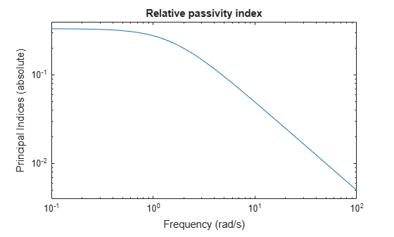
The plot shows that the relative passivity index is less than 1 at all frequencies. Therefore, the system G is passive.

Plot the input passivity index of the same system.

passiveplot(G,'input')

Figure contains an axes object. The axes object contains an object of type line. This object represents G.

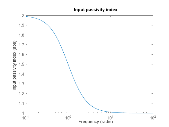
The input passivity index is positive at all frequencies. Therefore, the system is input strictly passive.

Plot the input passivity index of two dynamic systems and their series interconnection.

G1 = tf([5 3 1],[1 2 1]);
G2 = tf([1 1 5 0.1],[1 2 3 4]);
H = G2*G1;

passiveplot(G1,'r',G2,'b--',H,'gx','input')
legend('G1','G2','G2*G1')

Figure contains an axes object. The axes object contains 3 objects of type line. One or more of the lines displays its values using only markers These objects represent G1, G2, G2*G1.

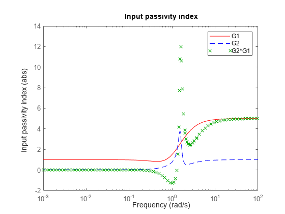
The input passivity index of the interconnected system dips below 0 around 1 rad/s. This plot shows that the series interconnection of two passive systems is not necessarily passive. However, passivity is preserved for parallel or feedback interconnections of passive systems.

Plot the relative passivity indices of a complex-coefficient model and a real-coefficient model on the same plot.

A = [-3.50,-1.25-0.25i;2,0];
B = [1;0];
C = [-0.75-0.5i,0.625-0.125i];
D = 0.5;
Gc = ss(A,B,C,D);
Gr = tf([1 5 10],[1 10 5]);
passiveplot(Gc,Gr)
legend('Complex-coefficient model','Real-coefficient model','Location','southeast')

Figure contains an axes object. The axes object contains 2 objects of type line. These objects represent Complex-coefficient model, Real-coefficient model.

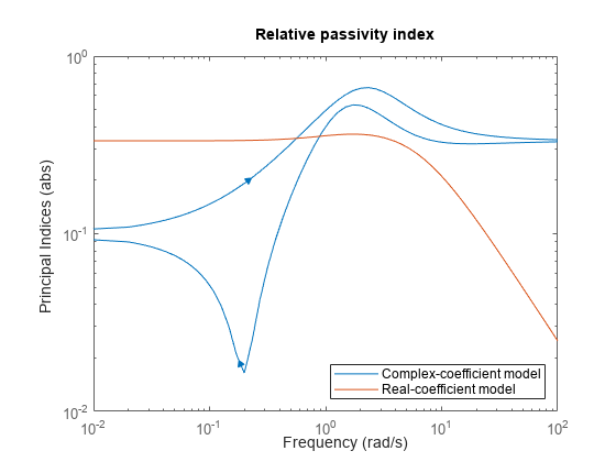
In log frequency scale, the plot shows two branches for models with complex coefficients, one for positive frequencies, with a right-pointing arrow, and one for negative frequencies, with a left-pointing arrow. In both branches, the arrows indicate the direction of increasing frequencies. The plots for models with real coefficients always contain a single branch with no arrows.

Set the plotting frequency scale to linear.

opt = sectorplotoptions;
opt.FreqScale = 'Linear';

Plot the indices.

passiveplot(Gc,Gr,opt)
legend('Complex-coefficient model','Real-coefficient model')

Figure contains an axes object. The axes object contains 2 objects of type line. These objects represent Complex-coefficient model, Real-coefficient model.

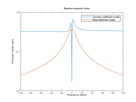
In linear frequency scale, the plots show a single branch with a symmetric frequency range centered at a frequency value of zero. The plot also shows the negative-frequency response of a real-coefficient model when you plot the response along with a complex-coefficient model.

Input Arguments

collapse all

Model to analyze for passivity, specified as a dynamic system model such as a tf, ss, or genss model. G can be MIMO, if the number of inputs equals the number of outputs. G can be continuous or discrete. If G is a generalized model with tunable or uncertain blocks, passiveplot evaluates passivity of the current, nominal value of G.

If G is a model array, then passiveplot plots the passivity index of all models in the array on the same plot. When you use output arguments to get passivity data, G must be a single model.

Type of passivity index, specified as one of the following:

  • 'input' — Input passivity index (input feedforward passivity). This value is the smallest eigenvalue of (G(s)+G(s)H)/2, for s = in continuous time, and s = e in discrete time.

  • 'output' — Output passivity index (output feedback passivity). When G is minimum phase, this value is the smallest eigenvalue of (G(s)1+G(s)H)/2, for s = in continuous time, and s = e in discrete time.

  • 'io' — Combined I/O passivity index. When I + G is minimum phase, this value is the largest τ(ω) such that:

    G(s)+G(s)H>2τ(ω)(I+G(s)HG(s)),

    for s = in continuous time, and s = e in discrete time.

See About Passivity and Passivity Indices for details about these indices.

Frequencies at which to compute and plot indices, specified as the cell array {wmin,wmax} or as a vector of frequency values.

  • If w is a cell array of the form {wmin,wmax}, then the function computes the index at frequencies ranging between wmin and wmax.

  • If w is a vector of frequencies, then the function computes the index at each specified frequency. For example, use logspace to generate a row vector with logarithmically-spaced frequency values.

For models with complex coefficients, if you specify a frequency range of [wmin,wmax] for your plot, then in:

  • Log frequency scale, the plot frequency limits are set to [wmin,wmax] and the plot shows two branches, one for positive frequencies [wmin,wmax] and one for negative frequencies [–wmax,–wmin].

  • Linear frequency scale, the plot frequency limits are set to [–wmax,wmax] and the plot shows a single branch with a symmetric frequency range centered at a frequency value of zero.

Specify frequencies in units of rad/TimeUnit, where TimeUnit is the TimeUnit property of the model.

Line style, marker, and color, specified as a string or vector of one, two, or three characters. The characters can appear in any order. You do not need to specify all three characteristics (line style, marker, and color). For example, if you omit the line style and specify the marker, then the plot shows only the marker and no line. For more information about configuring this argument, see the LineSpec input argument of the plot function.

Example: 'r--' specifies a red dashed line

Example: '*b' specifies blue asterisk markers

Example: 'y' specifies a yellow line

Passivity index plot options set, specified as a SectorPlotOptions object. You can use this option set to customize the plot appearance. Use sectorplotoptions to create the option set. Settings you specify in plotoptions overrides the preference settings in the MATLAB session in which you run passiveplot. Therefore, plotoptions is useful when you want to write a script to generate multiple plots that look the same regardless of the local preferences.

For the list of available options, see sectorplotoptions.

Output Arguments

collapse all

Passivity indices as a function of frequency, returned as a matrix. index contains whichever type of passivity index you specify, computed at the frequencies w if you supplied them, or wout if you did not. index has as many columns as there are values in w or wout, and

  • One row, for the input, output, or combined i/o passivity indices.

  • As many rows as G has inputs or outputs, for the relative passivity index.

For example, suppose that G is a 3-input, 3-output system, and w is a 1-by-30 vector of frequencies. Then the following syntax returns a 3-by-30 matrix index.

index = passiveplot(G,w);

The entry index(:,k) contains the relative passivity indices of G, in descending order, at the frequency w(k).

Frequencies at which the indices are calculated, returned as a vector. The function automatically chooses the frequency range and number of points based on the dynamics of the model.

wout also contains negative frequency values for models with complex coefficients.

Version History

Introduced in R2016a