Prune Filters in a Detection Network Using Taylor Scores
This example shows how to reduce network size and increase inference speed by pruning convolutional filters in a you only look once (YOLO) v3 object detection network.
Filter pruning is a compression technique that uses some criterion to identify and remove the least important filters in a network, reducing the overall memory footprint of the network without significant reduction in the network accuracy. The pruning algorithm used in this example is gradient-based and uses first-order Taylor expansion [1][2] to evaluate the importance of convolutional filters in a network. This example also shows how to generate code for the pruned network and deploy a processor-in-the-loop (PIL) executable to a Raspberry Pi® embedded target.
This example uses YOLO v3 detector trained on the Caltech Cars data set. For more information, see Object Detection Using YOLO v3 Deep Learning (Computer Vision Toolbox).
Load Network for Pruning
Load the trained network for pruning. The pretrained YOLO v3 detector in this example is based on SqueezeNet, and uses the feature extraction network in SqueezeNet with the addition of two detection heads at the end. The second detection head is twice the size of the first detection head, so it is better able to detect small objects.
For information on network training, see Object Detection Using YOLO v3 Deep Learning (Computer Vision Toolbox).
Download the yolov3SqueezeNetVehicleExample_21a.zip file containing the pretrained YOLO v3 network. This file is approximately 23MB in size. Download the file from the MathWorks® website, then unzip the file.
fileName = matlab.internal.examples.downloadSupportFile("vision/data/","yolov3SqueezeNetVehicleExample_21aSPKG.zip");
unzip(fileName);
matFile = "yolov3SqueezeNetVehicleExample_21aSPKG.mat";
pretrained = load(matFile);
yolov3Detector = pretrained.detector;
net = yolov3Detector.Network
net =
  dlnetwork with properties:

         Layers: [75×1 nnet.cnn.layer.Layer]
    Connections: [84×2 table]
     Learnables: [66×3 table]
          State: [6×3 table]
     InputNames: {'data'}
    OutputNames: {'customOutputConv1'  'customOutputConv2'}
    Initialized: 1

  View summary with summary.
Set random number generator for reproducibility.
rng(0);
Load and Prepare Vehicle Data
Load the training and validation data that will be used for pruning, fine-tuning, and retraining. This example uses a small labeled data set that contains 295 images. Many of these images come from the Caltech Cars 1999 and 2001 data sets, created by Pietro Perona and used with permission. Each image contains one or two labeled instances of a vehicle.
Unzip the vehicle images and load the vehicle ground truth data.
unzip("vehicleDatasetImages.zip");
data = load("vehicleDatasetGroundTruth.mat");
vehicleDataset = data.vehicleDataset;
Add the full path to the local vehicle data folder.
vehicleDataset.imageFilename = fullfile(pwd, vehicleDataset.imageFilename);
Split the data set into a training set for training the network, and a test set for evaluating the network. Use 60% of the data for training set and the rest for the test set.
shuffledIndices = randperm(height(vehicleDataset));
idx = floor(0.6 * length(shuffledIndices));
trainingDataTbl = vehicleDataset(shuffledIndices(1:idx), :);
testDataTbl = vehicleDataset(shuffledIndices(idx+1:end), :);
Create image and box label datastores.
imdsTrain = imageDatastore(trainingDataTbl.imageFilename);
imdsTest = imageDatastore(testDataTbl.imageFilename);
bldsTrain = boxLabelDatastore(trainingDataTbl(:, 2:end));
bldsTest = boxLabelDatastore(testDataTbl(:, 2:end));
trainingData = combine(imdsTrain, bldsTrain);
testData = combine(imdsTest, bldsTest);
Use validateInputData to detect invalid images, bounding boxes or labels. Any invalid samples must either be discarded or fixed for proper training.
validateInputData(trainingData);
validateInputData(testData);
Use the transform function to apply custom data augmentations to the training data. The augmentData helper function, listed at the end of the example, applies the following augmentations to the input data.
Color jitter augmentation in HSV space
Random horizontal flip
Random scaling by 10 percent
augmentedTrainingData = transform(trainingData, @augmentData);
Use transform to preprocess the training data for computing the anchor boxes, as the training images used in this example are bigger than 227-by-227 and vary in size. Then, use the estimateAnchorBoxes function to estimate the anchor boxes. Specify the number of anchors as 6 to achieve a good tradeoff between number of anchors and mean IoU. To prevent the estimated anchor boxes from changing while tuning other hyperparameters, the random seed is set prior to estimation using rng(0).
networkInputSize = [227 227 3];
trainingDataForEstimation = transform(trainingData, @(data)preprocessData(data, networkInputSize));
numAnchors = 6;
[anchorBoxes, meanIoU] = estimateAnchorBoxes(trainingDataForEstimation, numAnchors);
Specify anchorBoxes to use in both the detection heads. Select anchorBoxes for each detection head based on the feature map size. Use larger anchors at lower scale and smaller anchors at higher scale. To do so, sort the anchors with the larger anchor boxes first and assign the first three to the first detection head and the next three to the second detection head.
area = anchorBoxes(:, 1).*anchorBoxes(:, 2);
[~, idx] = sort(area, 'descend');
anchorBoxes = anchorBoxes(idx, :);
anchorBoxMasks = {[1,2,3] [4,5,6]};
classNames = trainingDataTbl.Properties.VariableNames(2:end);
Preprocess the augmented training data to prepare for training. The preprocessData helper function (defined at the end of this example) resizes the images to the network input size by maintaining the aspect ratio and scales the image pixels to the range [0 1].
augimdsTrain = transform(augmentedTrainingData, @(data)preprocessData(data, networkInputSize));
augimdsTest = transform(testData, @(data)preprocessData(data, networkInputSize));
Evaluate Detector Network Before Pruning
Use the evaluateObjectDetection (Computer Vision Toolbox) function to measure the average precision of the trained network before pruning. The average precision provides a single number that incorporates the ability of the detector to make correct classifications (precision) and the ability of the detector to find all relevant objects (recall).
results = detect(yolov3Detector,testData,MiniBatchSize=16);
Warning: Support for GPU devices with compute capability 6.1 will be removed in a future MATLAB release. For more information on GPU support, see <a href="matlab:web('http://www.mathworks.com/help/parallel-computing/gpu-computing-requirements.html','-browser')">GPU Computing Requirements</a>.
metrics = evaluateObjectDetection(results,testData);
apTrainedNet = metrics.ClassMetrics.AP{:};
recallTrainedNet = metrics.ClassMetrics.Recall{:};
precisionTrainedNet = metrics.ClassMetrics.Precision{:};
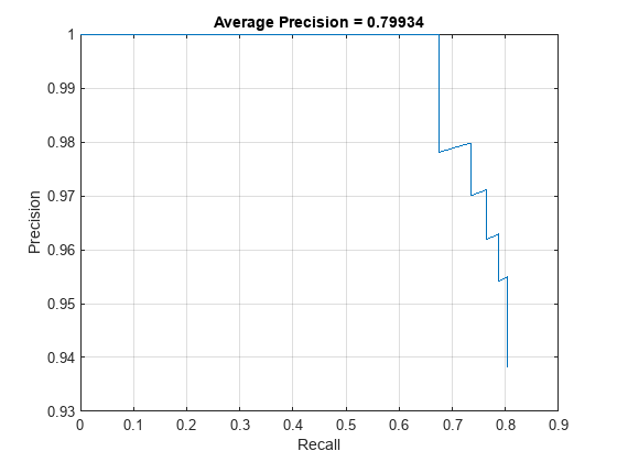
accuracyTrainedNet = mean(apTrainedNet)*100accuracyTrainedNet = 79.9338
The precision-recall (PR) curve shows how precise a detector is at varying levels of recall. Ideally, the precision is 1 at all recall levels.
figure
plot(recallTrainedNet,precisionTrainedNet)
xlabel("Recall")
ylabel("Precision")
xlim([0 1])
ylim([0.9 1])
grid on
title("Average Precision = " + apTrainedNet)
Prune Network
Create a prunable object based on first-order Taylor approximation by using taylorPrunableNetwork (Deep Learning Toolbox). A taylorPrunableNetwork has similar properties and methods as a dlnetwork in addition to pruning specific properties and methods. The prunable object can be substituted for a dlnetwork in the custom training loop. Pruning is iterative; each time the loop runs, until a stopping criterion is met, the function removes a small number of the least important convolution filters and updates the network architecture.
prunableNet = taylorPrunableNetwork(net)
prunableNet =
  TaylorPrunableNetwork with properties:

      Learnables: [66×3 table]
           State: [6×3 table]
      InputNames: {'data'}
     OutputNames: {'customOutputConv1'  'customOutputConv2'}
    NumPrunables: 3496
maxPrunableFilters = prunableNet.NumPrunables;
Specify Pruning Options
Set the pruning options.
maxPruningIterationsdefines the maximum number of iterations to be used in the pruning loop.maxToPruneis the maximum number of filters to be pruned in each iteration of the pruning loop.validationFrequencyis the number of iterations to wait before validating the pruned network using the test data.
maxPruningIterations = 20;
maxToPrune = 64;
validationFrequency = 5;
Set the fine-tuning options.
Fine-tune the network via a custom training loop for 40 mini-batches in every pruning iteration.
Specify the options for SGDM optimization. Specify an initial learn rate of 0.00001 and momentum of 0.9. Set the L2 regularization factor to 0.0005. Initialize the velocity of gradient as
[]. This is used by SGDM to store the velocity of gradients.Specify the penalty threshold as 0.5. Detections that overlap less than 0.5 with the ground truth are penalized.
Specify a mini-batch size of 16 to fine-tune the network.
numMinibatchUpdates = 40;
learnRate = 1e-5;
momentum = 0.9;
l2Regularization = 0.0005;
penaltyThreshold = 0.5;
miniBatchSize = 16;
Create Mini-Batch Queue
Use a minibatchqueue object to process and manage the mini-batches of images. For each mini-batch:
Use the custom mini-batch preprocessing function
preprocessMiniBatch(defined at the end of this example) which returns the batched images and bounding boxes combined with the respective class IDs.Format the image data with the dimension labels
'SSCB'(spatial, spatial, channel, batch). Do not add a format to the bounding boxes.Specify the data type of the bounding boxes.
mbq = minibatchqueue(augimdsTrain, 2,...
    MiniBatchSize=miniBatchSize,...
    MiniBatchFcn=@(images, boxes, labels) preprocessMiniBatch(images, boxes, labels, classNames), ...
    MiniBatchFormat=["SSCB", ""],...
    OutputCast=["", "double"]);
Prune Network Using Custom Pruning Loop
Initialize the training progress plots.
figure("Position",[10,10,700,700])
tl = tiledlayout(3,1);
lossAx = nexttile;
lineLossFinetune = animatedline(Color=[0.85 0.325 0.098]);
ylim([0 inf])
xlabel("Fine-Tuning Iteration")
ylabel("Loss")
grid on
title("Mini-Batch Loss during Pruning")
xTickPos = [];

accuracyAx = nexttile;
lineAccuracyPruning = animatedline(Color=[0.098 0.325 0.85]);
ylim([50 100])
xlabel("Pruning Iteration")
ylabel("Accuracy")
grid on
addpoints(lineAccuracyPruning, 0, accuracyTrainedNet)
title("Validation Accuracy After Pruning")

numPrunablesAx = nexttile;
lineNumPrunables = animatedline(Color=[0.4660 0.6470 0.1880]);
ylim([200 3600])
xlabel("Pruning Iteration")
ylabel("Prunable Filters")
grid on
addpoints(lineNumPrunables, 0, maxPrunableFilters)
title("Number of Prunable Convolution Filters After Pruning")
Prune the network. For each mini-batch in the pruning iteration, the following steps are used:
Evaluate the pruning activations, gradients of the pruning activations, model gradients, state, and loss using
dlfevalandmodelLossPruningfunctions.Update the network state.
Apply a weight decay factor to the gradients to regularization for more robust training.
Update the network learnable parameters using the stochastic gradient descent with momentum (SGDM) algorithm.
Compute first-order Taylor scores and accumulate the score across previous minibatches of data.
Display the progress.
In a loop, alternate between fine-tuning and pruning.
start = tic;
iteration = 0;

for pruningIteration = 1:maxPruningIterations

    % Shuffle the data in the minibatch.
    shuffle(mbq);

    % Reset the velocity parameter for the SGDM solver in every pruning
    % iteration.
    velocity = [];

    % Loop over mini-batches.
    fineTuningIteration = 0;
    while hasdata(mbq)
        iteration = iteration + 1;
        fineTuningIteration = fineTuningIteration + 1;

        % Read mini-batch of data.
        [X, T] = next(mbq);

        % Evaluate the pruning activations, gradients of the pruning
        % activations, model gradients, state, and loss using dlfeval and
        % modelLossPruning functions.
        [loss, pruningGradients, netGradients, pruningActivations, state] = ...
            dlfeval(@modelLossPruning, prunableNet, X, T, anchorBoxes, ...
            anchorBoxMasks, penaltyThreshold);

        % Update the network state.
        prunableNet.State = state;

        % Apply L2 regularization.
        netGradients = dlupdate(@(g,w) g + l2Regularization*w, ...
            netGradients, prunableNet.Learnables);

        % Update the network parameters using the SGDM optimizer.
        [prunableNet, velocity] = sgdmupdate(prunableNet, ...
            netGradients, velocity, learnRate, momentum);

        % Compute first-order Taylor scores and accumulate the score across
        % previous mini-batches of data.
        prunableNet = updateScore(prunableNet, pruningActivations, pruningGradients);

        % Display the training progress.
        D = duration(0,0,toc(start),'Format','hh:mm:ss');
        addpoints(lineLossFinetune, iteration, loss.totalLoss)
        title(tl,"Processing Pruning Iteration: " + pruningIteration + " of " + maxPruningIterations + ...
            ", Elapsed Time: " + string(D))
        % Synchronize the x-axis of the accuracy plot with the loss plot.
        xlim(accuracyAx,lossAx.XLim)
        xlim(numPrunablesAx,lossAx.XLim)
        drawnow

        % Stop the fine-tuning loop when numMinibatchUpdates is reached.
        if (fineTuningIteration > numMinibatchUpdates)
            break
        end

    end

    % Prune filters based on previously computed Taylor scores.
    prunableNet = updatePrunables(prunableNet, MaxToPrune = maxToPrune);

    % Show results on validation data set in a subset of pruning
    % iterations.
    isLastPruningIteration = pruningIteration == maxPruningIterations;
    if (mod(pruningIteration, validationFrequency) == 0 || isLastPruningIteration)
        [ap,~,~] = modelAccuracy(prunableNet, augimdsTest, anchorBoxes, anchorBoxMasks, classNames, 16);
        accuracy = mean(ap)*100;
        addpoints(lineAccuracyPruning, iteration, accuracy)
        addpoints(lineNumPrunables,iteration,prunableNet.NumPrunables)
    end

    % Set x-axis tick values at the end of each pruning iteration.
    xTickPos = [xTickPos, iteration];
    xticks(lossAx,xTickPos)
    xticks(accuracyAx,[0,xTickPos])
    xticks(numPrunablesAx,[0,xTickPos])
    xticklabels(accuracyAx,["Unpruned",string(1:pruningIteration)])
    xticklabels(numPrunablesAx,["Unpruned",string(1:pruningIteration)])
    drawnow
end
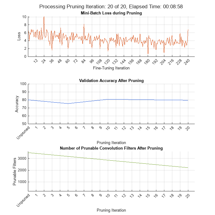
During each pruning iteration, the validation accuracy may reduce because of changes in the network structure when the convolutional filters are pruned. To minimize loss accuracy, it is recommended to retrain the network after pruning.
Once pruning is complete, convert the deep.prune.TaylorPrunableNetwork object back to a dlnetwork for retraining and further analysis.
prunedNet = dlnetwork(prunableNet);
save("prunedNet","prunedNet");
Retrain Pruned Network
The pruning process can cause the prediction accuracy to decrease. Try to improve the prediction accuracy by retraining the network using a custom training loop.
Specify Training Options
Specify the options to use during retraining.
Specify the options for SGDM optimization. Specify an initial learn rate of 0.0001 and momentum of 0.9. Set the L2 regularization factor to 0.0005. Initialize the velocity of gradient as
[]. This is used by SGDM to store the velocity of gradients.Use the custom mini-batch preprocessing function
preprocessMiniBatch(defined at the end of this example) which returns the batched images and bounding boxes combined with the respective class IDs.Format the image data with the dimension labels
'SSCB'(spatial, spatial, channel, batch). Do not add a format to the bounding boxes.Specify the data type of the bounding boxes.
learnRate = 1e-4;
velocity = [];
momentum = 0.9;
numEpochs = 10;
l2Regularization = 0.0005;
mbq = minibatchqueue(augimdsTrain, 2,...
    MiniBatchSize=miniBatchSize,...
    MiniBatchFcn=@(images, boxes, labels) preprocessMiniBatch(images, boxes, labels, classNames), ...
    MiniBatchFormat=["SSCB", ""],...
    OutputCast=["", "double"]);
Train Network Using Custom Training Loop
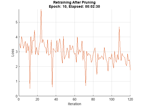
Initialize the training progress plot.
figure
lineLossTrain = animatedline('Color',[0.85 0.325 0.098]);
ylim([0 inf])
xlabel("Iteration")
ylabel("Loss")
grid on
For each epoch, loop over mini-batches while data is still available in the minibatchqueue. Update the network parameters using the SGDM algorithm.
iteration = 0;
start = tic;
prunedDetectorNet = prunedNet;

for i = 1:numEpochs
    % Shuffle the data in the minibatch.
    shuffle(mbq);

    % Loop over mini-batches.
    while hasdata(mbq)
        iteration = iteration + 1;

        % Read mini-batch of data.
        [X, T] = next(mbq);

        % Evaluate the model gradients, state, and loss using dlfeval and the
        % modelGradients function and update the network state.
        [loss, gradients, state] = dlfeval(@modelLossTraining, prunedDetectorNet,...
            X, T, anchorBoxes, anchorBoxMasks, penaltyThreshold);

        % Update the network state.
        prunedDetectorNet.State = state;

        % Apply L2 regularization.
        gradients = dlupdate(@(g,w) g + l2Regularization*w, gradients, prunedDetectorNet.Learnables);

        % Update the network parameters using the SGDM optimizer.
        [prunedDetectorNet, velocity] = sgdmupdate(prunedDetectorNet, gradients, velocity, learnRate, momentum);

        % Display the training progress.
        D = duration(0,0,toc(start),'Format','hh:mm:ss');
        addpoints(lineLossTrain,iteration,loss.totalLoss)
        title("Retraining After Pruning" + newline + "Epoch: " + numEpochs + ", Elapsed: " + string(D))
        drawnow
    end
end
prunedyolov3ObjectDetector = yolov3ObjectDetector(prunedDetectorNet,classNames,yolov3Detector.AnchorBoxes);
save("prunedyolov3","prunedyolov3ObjectDetector");
Compare Original Network and Pruned Network
Determine the impact of pruning on each layer.
originalNetFilters = numConvLayerFilters(net);
prunedNetFilters = numConvLayerFilters(prunedDetectorNet);
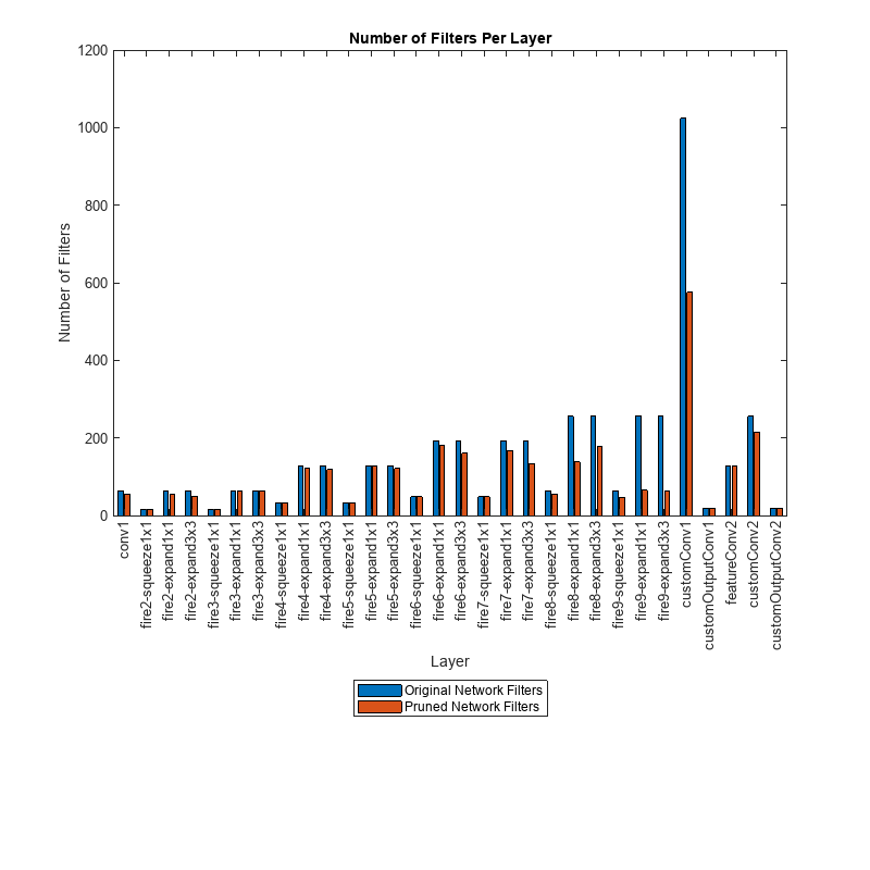
convFilters = join(originalNetFilters,prunedNetFilters,Keys="Row");Visualize the number of filters in the original network and in the pruned network.
figure("Position",[10,10,900,900])
bar([convFilters.(1),convFilters.(2)])
xlabel("Layer")
ylabel("Number of Filters")
title("Number of Filters Per Layer")
xticks(1:(numel(convFilters.Row)))
xticklabels(convFilters.Row)
xtickangle(90)
ax = gca;
ax.TickLabelInterpreter = "none";
legend("Original Network Filters","Pruned Network Filters","Location","southoutside")
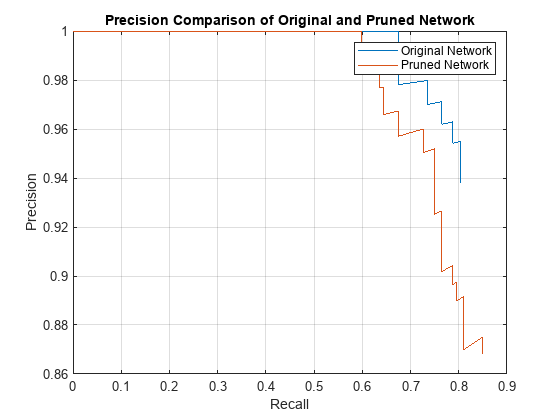
Next, compare the accuracy of the original network and the pruned network. The average precision provides a single number that incorporates the ability of the detector to make correct classifications (precision) and the ability of the detector to find all relevant objects (recall).
[apPrunedNet,recallPrunedNet,precisionPrunedNet] = modelAccuracy(prunedDetectorNet, augimdsTest, anchorBoxes, anchorBoxMasks, classNames, 16);
accuracyPrunedNet = mean(apPrunedNet)*100
accuracyPrunedNet =
85.9193
The precision-recall (PR) curve is a good way to evaluate the performance of the object detector. Ideally the precision is 1 for all levels of recall. The pruned object detector has lost some precision but can still be considered good as its precision stays high when the recall increases.
figure
plot(recallTrainedNet,precisionTrainedNet,recallPrunedNet,precisionPrunedNet)
xlabel("Recall")
ylabel("Precision")
xlim([0 1])
ylim([0.9 1])
grid on
title("Precision Comparison of Original and Pruned Network")
legend("Original Network","Pruned Network","Location","southwest");
Next, estimate the model parameters for the original network and the pruned network to understand the impact of pruning on the overall network learnables and size.
analyzeNetworkMetrics(net,prunedDetectorNet,accuracyTrainedNet,accuracyPrunedNet)
ans=3×3 table
     6415844     24.4745    79.9338
     1793585      6.8420    85.9193
    -72.0444    -72.0444     7.4880
Deploy Pruned YOLOv3 Network to Raspberry Pi
Optionally, you can use MATLAB® Coder™ to generate C++ code for the pruned network taking advantage of the ARM® Compute Library. The generated code can be integrated into your project as source code, static or dynamic libraries, or an executable that you can deploy to a variety of ARM CPU platforms such as Raspberry Pi. This example uses the PIL based workflow to generate a MEX function, which in turn calls the executable generated on a Raspberry Pi from MATLAB.
Third-Party Prerequisites
Raspberry Pi hardware
ARM Compute Library (on the target ARM hardware)
Environment variables for the compilers and libraries. For information on the supported versions of the compilers and libraries, see Generate Code That Uses Third-Party Libraries. For setting up the environment variables, see Environment Variables.
PIL MEX Function
In this example, you generate code for the entry-point function yolov3Raspi. This function uses the coder.loadDeepLearningNetwork function to load a deep learning model and to construct and set up a CNN class. Then the entry-point function detects vehicles in the input and returns an output image displaying the detections.
type yolov3Raspi.mfunction outImg = yolov3Raspi(in,matFile)
% Copyright 2022 The MathWorks, Inc.
persistent yolov3Obj;
if isempty(yolov3Obj)
yolov3Obj = coder.loadDeepLearningNetwork(matFile);
end
% Call to detect method.
[bboxes,~,labels] = detect(yolov3Obj,in,'Threshold',0.5);
% Convert categorical labels to cell array of charactor vectors.
labels = cellstr(labels);
% Annotate detections in the image.
outImg = insertObjectAnnotation(in,'rectangle',bboxes,labels);
To generate a PIL MEX function, create a code configuration object for a static library and set the verification mode to 'PIL'. Set the target language to C++.
cfg = coder.config("lib",ecoder=true);
cfg.VerificationMode = "PIL";
cfg.TargetLang = "C++";
Create a deep learning configuration object for the ARM Compute library. Specify the library version and ARM architecture. For this example, suppose that the ARM Compute Library in the Raspberry Pi hardware is version 20.02.1.
dlcfg = coder.DeepLearningConfig("arm-compute");
dlcfg.ArmComputeVersion = "20.02.1";
dlcfg.ArmArchitecture = "armv7";
Set the DeepLearningConfig property of cfg to dlcfg.
cfg.DeepLearningConfig = dlcfg;
Use the Raspberry Pi® Blockset function, raspi, to create a connection to the Raspberry Pi. In the following code, replace:
raspinamewith the name of your Raspberry Piusernamewith your user namepasswordwith your password
r = raspi("raspiname","username","password");
Then, create a coder.Hardware object for Raspberry Pi and attach it to the code generation configuration object.
hw = coder.hardware("Raspberry Pi");
cfg.Hardware = hw;
Generate a PIL MEX function for the original network in yolov3SqueezeNetVehicleExample_21aSPKG.mat by using the codegen command.
codegen -config cfg yolov3Raspi -args {ones(227,227,3,'single'),coder.Constant("yolov3SqueezeNetVehicleExample_21aSPKG.mat")}
Read a sample image and call the generated PIL MEX function yolov3Raspi_pil. The PIL MEX function launches the yolov3Raspi.elf executable on the Raspberry Pi and returns the results of the execution to MATLAB.
data = read(augimdsTest);
I = data{1};
tic;
detectedImage = yolov3Raspi_pil(I,"yolov3SqueezeNetVehicleExample_21aSPKG.mat");
execTimeOriginalNet = toc;
clear yolov3Raspi_pil;
imshow(detectedImage);
title("Execution Time of Original Network = "+execTimeOriginalNet+"s");
saveas(gcf,"DetectionResultsOriginalNet.png");
close(gcf);
imshow("DetectionResultsOriginalNet.png");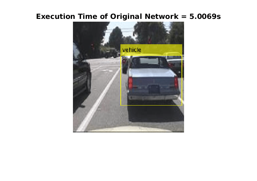
Then, generate a PIL MEX function for the pruned network in prunedyolov3.mat by using the codegen command.
codegen -config cfg yolov3Raspi -args {ones(227,227,3,'single'),coder.Constant("prunedyolov3.mat")}
Run the generated PIL MEX.
tic;
detectedImage = yolov3Raspi_pil(I,"prunedyolov3.mat");
execTimeOriginalNet = toc;
clear yolov3Raspi_pil
imshow(detectedImage);
title("Execution Time of Pruned Network = "+execTimeOriginalNet+"s");
saveas(gcf,"DetectionResultsPrunedNet.png");
close(gcf);
imshow("DetectionResultsPrunedNet.png");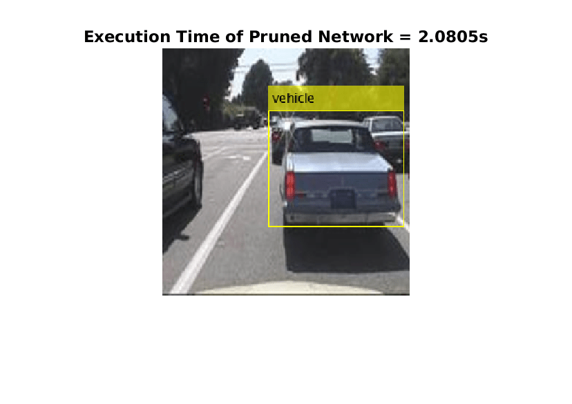
Helper Functions
Model Gradients Function for Fine-Tuning and Pruning
The function modelLossPruning takes as input a deep.prune.TaylorPrunableNetwork object prunableNet, a mini-batch of input data X with corresponding ground truth boxes T, anchor boxes, masks, penalty threshold and returns the loss, the gradients of the loss with respect to the pruning activations, gradients of loss with respect to the learnable parameters in prunableNet, pruning activations, and the network state.
function [loss, pruningGradients, netGradients, pruningActivations, state] = modelLossPruning(prunableNet, X, T, anchors, mask, penaltyThreshold)

inputImageSize = size(X,1:2);

% Gather the ground truths for post processing.
YTrain = gather(extractdata(T));

% Extract the predictions from the network.
[YPredCell, state, pruningActivations] = yolov3ForwardPrunable(prunableNet, X, mask);

% Gather the activations for post processing and extract dlarray data.
gatheredPredictions = cellfun(@ gather, YPredCell(:,1:6),'UniformOutput',false);
gatheredPredictions = cellfun(@ extractdata, gatheredPredictions, 'UniformOutput', false);

% Convert predictions from grid cell coordinates to box coordinates.
tiledAnchors = generateTiledAnchors(gatheredPredictions(:,2:5),anchors,mask);
gatheredPredictions(:,2:5) = applyAnchorBoxOffsets(tiledAnchors, gatheredPredictions(:,2:5), inputImageSize);

% Generate target for predictions from the ground truth data.
[boxTarget, objectnessTarget, classTarget, objectMaskTarget, boxErrorScale] = generateTargets(gatheredPredictions, YTrain, inputImageSize, anchors, mask, penaltyThreshold);

% Compute the loss.
boxLoss = bboxOffsetLoss(YPredCell(:,[2 3 7 8]),boxTarget,objectMaskTarget,boxErrorScale);
objLoss = objectnessLoss(YPredCell(:,1),objectnessTarget,objectMaskTarget);
clsLoss = classConfidenceLoss(YPredCell(:,6),classTarget,objectMaskTarget);
totalLoss = boxLoss + objLoss + clsLoss;

loss.boxLoss = boxLoss;
loss.objLoss = objLoss;
loss.clsLoss = clsLoss;
loss.totalLoss = totalLoss;

% Differentiate loss w.r.t learnables and activations
[netGradients, pruningGradients] = dlgradient(totalLoss, prunableNet.Learnables, pruningActivations);

end
Model Gradients Function for Retraining
The function modelLossTraining takes as input a dlnetwork object net, a mini-batch of input data X with corresponding ground truth boxes T, anchor boxes, masks, penalty threshold and returns the loss, gradients of loss with respect to the learnable parameters in net, and the network state.
function [loss, gradients, state] = modelLossTraining(net, X, T, anchors, mask, penaltyThreshold)

inputImageSize = size(X,1:2);

% Gather the ground truths for post processing.
YTrain = gather(extractdata(T));

% Extract the predictions from the network.
[YPredCell, state] = yolov3Forward(net,X,mask);

% Gather the activations for post processing and extract dlarray data.
gatheredPredictions = cellfun(@ gather, YPredCell(:,1:6),'UniformOutput',false);
gatheredPredictions = cellfun(@ extractdata, gatheredPredictions, 'UniformOutput', false);

% Convert predictions from grid cell coordinates to box coordinates.
tiledAnchors = generateTiledAnchors(gatheredPredictions(:,2:5),anchors,mask);
gatheredPredictions(:,2:5) = applyAnchorBoxOffsets(tiledAnchors, gatheredPredictions(:,2:5), inputImageSize);

% Generate target for predictions from the ground truth data.
[boxTarget, objectnessTarget, classTarget, objectMaskTarget, boxErrorScale] = generateTargets(gatheredPredictions, YTrain, inputImageSize, anchors, mask, penaltyThreshold);

% Compute the loss.
boxLoss = bboxOffsetLoss(YPredCell(:,[2 3 7 8]),boxTarget,objectMaskTarget,boxErrorScale);
objLoss = objectnessLoss(YPredCell(:,1),objectnessTarget,objectMaskTarget);
clsLoss = classConfidenceLoss(YPredCell(:,6),classTarget,objectMaskTarget);
totalLoss = boxLoss + objLoss + clsLoss;

loss.boxLoss = boxLoss;
loss.objLoss = objLoss;
loss.clsLoss = clsLoss;
loss.totalLoss = totalLoss;

% Differentiate loss w.r.t learnables
gradients = dlgradient(totalLoss, net.Learnables);

end
Mini-Batch Preprocessing Function
The preprocessMiniBatch function preprocesses a mini-batch of data and returns the batched images and bounding boxes combined with the respective class IDs.
function [X, T] = preprocessMiniBatch(data, groundTruthBoxes, groundTruthClasses, classNames)
% Returns images combined along the batch dimension in XTrain and
% normalized bounding boxes concatenated with classIDs in YTrain.

% Concatenate images along the batch dimension.
X = cat(4, data{:,1});

% Get class IDs from the class names.
classNames = repmat({categorical(classNames')}, size(groundTruthClasses));
[~, classIndices] = cellfun(@(a,b)ismember(a,b), groundTruthClasses, classNames, 'UniformOutput', false);

% Append the label indexes and training image size to scaled bounding boxes
% and create a single cell array of responses.
combinedResponses = cellfun(@(bbox, classid)[bbox, classid], groundTruthBoxes, classIndices, 'UniformOutput', false);
len = max( cellfun(@(x)size(x,1), combinedResponses ) );
paddedBBoxes = cellfun( @(v) padarray(v,[len-size(v,1),0],0,'post'), combinedResponses, 'UniformOutput',false);
T = cat(4, paddedBBoxes{:,1});
end
Evaluate Model Accuracy
The modelAccuracy computes the accuracy of the network on the data set.
function [ap, recall, precision] = modelAccuracy(net, augimds, anchorBoxes, anchorBoxMasks, classNames, miniBatchSize)
% Computes model accuracy on the dataset 'augimds'.

% Create a table to hold the bounding boxes, scores, and labels returned by
% the detector.
results = table('Size', [0 3], ...
    'VariableTypes', {'cell','cell','cell'}, ...
    'VariableNames', {'Boxes','Scores','Labels'});
mbqTest = minibatchqueue(augimds, 1, ...
    "MiniBatchSize", miniBatchSize, ...
    "MiniBatchFormat", "SSCB");

% Run detector on images in the test set and collect results.
while hasdata(mbqTest)
    % Read the datastore and get the image.
    XTest = next(mbqTest);

    % Run the detector.
    [bboxes, scores, labels] = yolov3Detect(net, XTest, net.OutputNames', anchorBoxes, anchorBoxMasks, 0.5, 0.5, classNames);

    % Collect the results.
    tbl = table(bboxes, scores, labels, 'VariableNames', {'Boxes','Scores','Labels'});
    results = [results; tbl];
end

% Evaluate the object detector using Average Precision metric.
metrics = evaluateObjectDetection(results,augimds);
ap = metrics.ClassMetrics.AP{:};
recall = metrics.ClassMetrics.Recall{:};
precision = metrics.ClassMetrics.Precision{:};
end
Evaluate Number of Filters in Convolution Layers
The numConvLayerFilters function returns the number of filters in each convolution layer.
function convFilters = numConvLayerFilters(net)
numLayers = numel(net.Layers);
convNames = [];
numFilters = [];
% Check for convolution layers and extract the number of filters.
for cnt = 1:numLayers
    if isa(net.Layers(cnt),"nnet.cnn.layer.Convolution2DLayer")
        sizeW = size(net.Layers(cnt).Weights);
        numFilters = [numFilters; sizeW(end)];
        convNames = [convNames; string(net.Layers(cnt).Name)];
    end
end
convFilters = table(numFilters,RowNames=convNames);
end
Evaluate the Network Statistics of Original Network and Pruned Network
The analyzeNetworkMetrics function takes input as the original network, pruned network, accuracy of original network and the accuracy of the pruned network and returns the different statistics like network learnables, network memory, and the accuracy on the test data in form of a table.
function [statistics] = analyzeNetworkMetrics(originalNet,prunedNet,accuracyOriginal,accuracyPruned)

originalNetMetrics = estimateNetworkMetrics(originalNet);
prunedNetMetrics = estimateNetworkMetrics(prunedNet);

% Accuracy of original network and pruned network
perChangeAccu = 100*(accuracyPruned - accuracyOriginal)/accuracyOriginal;
AccuracyForNetworks = [accuracyOriginal;accuracyPruned;perChangeAccu];

% Total learnables in both networks
originalNetLearnables = sum(originalNetMetrics(1:end,"NumberOfLearnables").NumberOfLearnables);
prunedNetLearnables = sum(prunedNetMetrics(1:end,"NumberOfLearnables").NumberOfLearnables);
percentageChangeLearnables = 100*(prunedNetLearnables - originalNetLearnables)/originalNetLearnables;
LearnablesForNetwork = [originalNetLearnables;prunedNetLearnables;percentageChangeLearnables];

% Approximate parameter memory
approxOriginalMemory = sum(originalNetMetrics(1:end,"ParameterMemory (MB)").("ParameterMemory (MB)"));
approxPrunedMemory = sum(prunedNetMetrics(1:end,"ParameterMemory (MB)").("ParameterMemory (MB)"));
percentageChangeMemory = 100*(approxPrunedMemory - approxOriginalMemory)/approxOriginalMemory;
NetworkMemory = [ approxOriginalMemory; approxPrunedMemory; percentageChangeMemory];

% Create the summary table
statistics = table(LearnablesForNetwork,NetworkMemory,AccuracyForNetworks, ...
    'VariableNames',["Network Learnables","Approx. Network Memory (MB)","Accuracy"], ...
    'RowNames',{'Original Network','Pruned Network','Percentage Change'});

end
Augmentation and Data Processing Functions
function data = augmentData(A)
% Apply random horizontal flipping, and random X/Y scaling. Boxes that get
% scaled outside the bounds are clipped if the overlap is above 0.25. Also,
% jitter image color.
data = cell(size(A));
for ii = 1:size(A,1)
    I = A{ii,1};
    bboxes = A{ii,2};
    labels = A{ii,3};
    sz = size(I);

    if numel(sz) == 3 && sz(3) == 3
        I = jitterColorHSV(I,...
            'Contrast',0.0,...
            'Hue',0.1,...
            'Saturation',0.2,...
            'Brightness',0.2);
    end

    % Randomly flip image.
    tform = randomAffine2d('XReflection',true,'Scale',[1 1.1]);
    rout = affineOutputView(sz,tform,'BoundsStyle','centerOutput');
    I = imwarp(I,tform,'OutputView',rout);

    % Apply same transform to boxes.
    [bboxes,indices] = bboxwarp(bboxes,tform,rout,'OverlapThreshold',0.25);
    bboxes = round(bboxes);
    labels = labels(indices);

    % Return original data only when all boxes are removed by warping.
    if isempty(indices)
        data(ii,:) = A(ii,:);
    else
        data(ii,:) = {I, bboxes, labels};
    end
end
end

function data = preprocessData(data, targetSize)
% Resize the images and scale the pixels to between 0 and 1. Also scale the
% corresponding bounding boxes.
for ii = 1:size(data,1)
    I = data{ii,1};
    imgSize = size(I);

    % Convert an input image with single channel to 3 channels.
    if numel(imgSize) < 3
        I = repmat(I,1,1,3);
    end
    bboxes = data{ii,2};

    I = im2single(imresize(I,targetSize(1:2)));
    scale = targetSize(1:2)./imgSize(1:2);
    bboxes = bboxresize(bboxes,scale);

    data(ii, 1:2) = {I, bboxes};
end
end
Utility Functions
function YPredCell = applyActivations(YPredCell)
% Apply activation functions on YOLOv3 outputs.
YPredCell(:,1:3) = cellfun(@ sigmoid, YPredCell(:,1:3), 'UniformOutput', false);
YPredCell(:,4:5) = cellfun(@ exp, YPredCell(:,4:5), 'UniformOutput', false);
YPredCell(:,6) = cellfun(@ sigmoid, YPredCell(:,6), 'UniformOutput', false);
end

function tiledAnchors = applyAnchorBoxOffsets(tiledAnchors,YPredCell,inputImageSize)
% Convert grid cell coordinates to box coordinates.
for i=1:size(YPredCell,1)
    [h,w,~,~] = size(YPredCell{i,1});
    tiledAnchors{i,1} = (tiledAnchors{i,1}+YPredCell{i,1})./w;
    tiledAnchors{i,2} = (tiledAnchors{i,2}+YPredCell{i,2})./h;
    tiledAnchors{i,3} = (tiledAnchors{i,3}.*YPredCell{i,3})./inputImageSize(2);
    tiledAnchors{i,4} = (tiledAnchors{i,4}.*YPredCell{i,4})./inputImageSize(1);
end
end

function boxLoss = bboxOffsetLoss(boxPredCell, boxDeltaTarget, boxMaskTarget, boxErrorScaleTarget)
% Mean squared error for bounding box position.
lossX = sum(cellfun(@(a,b,c,d) mse(a.*c.*d,b.*c.*d),boxPredCell(:,1),boxDeltaTarget(:,1),boxMaskTarget(:,1),boxErrorScaleTarget));
lossY = sum(cellfun(@(a,b,c,d) mse(a.*c.*d,b.*c.*d),boxPredCell(:,2),boxDeltaTarget(:,2),boxMaskTarget(:,1),boxErrorScaleTarget));
lossW = sum(cellfun(@(a,b,c,d) mse(a.*c.*d,b.*c.*d),boxPredCell(:,3),boxDeltaTarget(:,3),boxMaskTarget(:,1),boxErrorScaleTarget));
lossH = sum(cellfun(@(a,b,c,d) mse(a.*c.*d,b.*c.*d),boxPredCell(:,4),boxDeltaTarget(:,4),boxMaskTarget(:,1),boxErrorScaleTarget));
boxLoss = lossX+lossY+lossW+lossH;
end

function clsLoss = classConfidenceLoss(classPredCell, classTarget, boxMaskTarget)
% Binary cross-entropy loss for class confidence score.
clsLoss = sum(cellfun(@(a,b,c) crossentropy(a.*c,b.*c,'ClassificationMode','multilabel'),classPredCell,classTarget,boxMaskTarget(:,3)));
end

function predictions = extractPredictions(YPredictions, anchorBoxMask)
% Function extractPrediction extracts and rearranges the prediction outputs
% from YOLOv3 network.

predictions = cell(size(YPredictions, 1),6);
for ii = 1:size(YPredictions, 1)
    % Get the required info on feature size.
    numChannelsPred = size(YPredictions{ii},3);
    numAnchors = size(anchorBoxMask{ii},2);
    numPredElemsPerAnchors = numChannelsPred/numAnchors;
    allIds = (1:numChannelsPred);

    stride = numPredElemsPerAnchors;
    endIdx = numChannelsPred;

    % X positions.
    startIdx = 1;
    predictions{ii,2} = YPredictions{ii}(:,:,startIdx:stride:endIdx,:);
    xIds = startIdx:stride:endIdx;

    % Y positions.
    startIdx = 2;
    predictions{ii,3} = YPredictions{ii}(:,:,startIdx:stride:endIdx,:);
    yIds = startIdx:stride:endIdx;

    % Width.
    startIdx = 3;
    predictions{ii,4} = YPredictions{ii}(:,:,startIdx:stride:endIdx,:);
    wIds = startIdx:stride:endIdx;

    % Height.
    startIdx = 4;
    predictions{ii,5} = YPredictions{ii}(:,:,startIdx:stride:endIdx,:);
    hIds = startIdx:stride:endIdx;

    % Confidence scores.
    startIdx = 5;
    predictions{ii,1} = YPredictions{ii}(:,:,startIdx:stride:endIdx,:);
    confIds = startIdx:stride:endIdx;

    % Accumulate all the non-class indexes
    nonClassIds = [xIds yIds wIds hIds confIds];

    % Class probabilities. Get the indexes which do not belong to the
    % nonClassIds
    classIdx = setdiff(allIds,nonClassIds);
    predictions{ii,6} = YPredictions{ii}(:,:,classIdx,:);
end
end

function [boxDeltaTarget, objectnessTarget, classTarget, maskTarget, boxErrorScaleTarget] = generateTargets(YPredCellGathered, groundTruth, inputImageSize, anchorBoxes, anchorBoxMask, penaltyThreshold)
% generateTargets creates target array for every prediction element
% x, y, width, height, confidence scores and class probabilities.
boxDeltaTarget = cell(size(YPredCellGathered,1),4);
objectnessTarget = cell(size(YPredCellGathered,1),1);
classTarget = cell(size(YPredCellGathered,1),1);
maskTarget = cell(size(YPredCellGathered,1),3);
boxErrorScaleTarget = cell(size(YPredCellGathered,1),1);

% Normalize the ground truth boxes w.r.t image input size.
gtScale = [inputImageSize(2) inputImageSize(1) inputImageSize(2) inputImageSize(1)];
groundTruth(:,1:4,:,:) = groundTruth(:,1:4,:,:)./gtScale;

for numPred = 1:size(YPredCellGathered,1)

    % Select anchor boxes based on anchor box mask indices.
    anchors = anchorBoxes(anchorBoxMask{numPred},:);

    bx = YPredCellGathered{numPred,2};
    by = YPredCellGathered{numPred,3};
    bw = YPredCellGathered{numPred,4};
    bh = YPredCellGathered{numPred,5};
    predClasses = YPredCellGathered{numPred,6};

    gridSize = size(bx);
    if numel(gridSize)== 3
        gridSize(4) = 1;
    end
    numClasses = size(predClasses,3)/size(anchors,1);

    % Initialize the required variables.
    mask = single(zeros(size(bx)));
    confMask = single(ones(size(bx)));
    classMask = single(zeros(size(predClasses)));
    tx = single(zeros(size(bx)));
    ty = single(zeros(size(by)));
    tw = single(zeros(size(bw)));
    th = single(zeros(size(bh)));
    tconf = single(zeros(size(bx)));
    tclass = single(zeros(size(predClasses)));
    boxErrorScale = single(ones(size(bx)));

    % Get the IOU of predictions with ground truth.
    iou = getMaxIOUPredictedWithGroundTruth(bx,by,bw,bh,groundTruth);

    % Do not penalize the predictions which have iou greater than penalty
    % threshold.
    confMask(iou > penaltyThreshold) = 0;

    for batch = 1:gridSize(4)
        truthBatch = groundTruth(:,1:5,:,batch);
        truthBatch = truthBatch(all(truthBatch,2),:);

        % Get boxes with center as 0.
        gtPred = [0-truthBatch(:,3)/2,0-truthBatch(:,4)/2,truthBatch(:,3),truthBatch(:,4)];
        anchorPrior = [0-anchorBoxes(:,2)/(2*inputImageSize(2)),0-anchorBoxes(:,1)/(2*inputImageSize(1)),anchorBoxes(:,2)/inputImageSize(2),anchorBoxes(:,1)/inputImageSize(1)];

        % Get the iou of best matching anchor box.
        overLap = bboxOverlapRatio(gtPred,anchorPrior);
        [~,bestAnchorIdx] = max(overLap,[],2);

        % Select gt that are within the mask.
        index = ismember(bestAnchorIdx,anchorBoxMask{numPred});
        truthBatch = truthBatch(index,:);
        bestAnchorIdx = bestAnchorIdx(index,:);
        bestAnchorIdx = bestAnchorIdx - anchorBoxMask{numPred}(1,1) + 1;

        if ~isempty(truthBatch)
            % Convert top left position of ground-truth to center coordinates.
            truthBatch = [truthBatch(:,1)+truthBatch(:,3)./2,truthBatch(:,2)+truthBatch(:,4)./2,truthBatch(:,3),truthBatch(:,4),truthBatch(:,5)];

            errorScale = 2 - truthBatch(:,3).*truthBatch(:,4);
            truthBatch = [truthBatch(:,1)*gridSize(2),truthBatch(:,2)*gridSize(1),truthBatch(:,3)*inputImageSize(2),truthBatch(:,4)*inputImageSize(1),truthBatch(:,5)];
            for t = 1:size(truthBatch,1)

                % Get the position of ground-truth box in the grid.
                colIdx = ceil(truthBatch(t,1));
                colIdx(colIdx<1) = 1;
                colIdx(colIdx>gridSize(2)) = gridSize(2);
                rowIdx = ceil(truthBatch(t,2));
                rowIdx(rowIdx<1) = 1;
                rowIdx(rowIdx>gridSize(1)) = gridSize(1);
                pos = [rowIdx,colIdx];
                anchorIdx = bestAnchorIdx(t,1);

                mask(pos(1,1),pos(1,2),anchorIdx,batch) = 1;
                confMask(pos(1,1),pos(1,2),anchorIdx,batch) = 1;

                % Calculate the shift in ground truth boxes.
                tShiftX = truthBatch(t,1)-pos(1,2)+1;
                tShiftY = truthBatch(t,2)-pos(1,1)+1;
                tShiftW = log(truthBatch(t,3)/anchors(anchorIdx,2));
                tShiftH = log(truthBatch(t,4)/anchors(anchorIdx,1));

                % Update the target box.
                tx(pos(1,1),pos(1,2),anchorIdx,batch) = tShiftX;
                ty(pos(1,1),pos(1,2),anchorIdx,batch) = tShiftY;
                tw(pos(1,1),pos(1,2),anchorIdx,batch) = tShiftW;
                th(pos(1,1),pos(1,2),anchorIdx,batch) = tShiftH;
                boxErrorScale(pos(1,1),pos(1,2),anchorIdx,batch) = errorScale(t);
                tconf(rowIdx,colIdx,anchorIdx,batch) = 1;
                classIdx = (numClasses*(anchorIdx-1))+truthBatch(t,5);
                tclass(rowIdx,colIdx,classIdx,batch) = 1;
                classMask(rowIdx,colIdx,(numClasses*(anchorIdx-1))+(1:numClasses),batch) = 1;
            end
        end
    end
    boxDeltaTarget(numPred,:) = [{tx} {ty} {tw} {th}];
    objectnessTarget{numPred,1} = tconf;
    classTarget{numPred,1} = tclass;
    maskTarget(numPred,:) = [{mask} {confMask} {classMask}];
    boxErrorScaleTarget{numPred,:} = boxErrorScale;
end
end

function iou = getMaxIOUPredictedWithGroundTruth(predx,predy,predw,predh,truth)
% getMaxIOUPredictedWithGroundTruth computes the maximum intersection over
% union scores for every pair of predictions and ground truth boxes.

[h,w,c,n] = size(predx);
iou = zeros([h w c n],'like',predx);

% For each batch, prepare the predictions and ground truth.
for batchSize = 1:n
    truthBatch = truth(:,1:4,1,batchSize);
    truthBatch = truthBatch(all(truthBatch,2),:);
    predxb = predx(:,:,:,batchSize);
    predyb = predy(:,:,:,batchSize);
    predwb = predw(:,:,:,batchSize);
    predhb = predh(:,:,:,batchSize);
    predb = [predxb(:),predyb(:),predwb(:),predhb(:)];

    % Convert from center xy coordinate to top left xy coordinate.
    predb = [predb(:,1)-predb(:,3)./2, predb(:,2)-predb(:,4)./2, predb(:,3), predb(:,4)];

    % Compute and extract the maximum IOU of predictions with ground truth.
    try
        overlap = bboxOverlapRatio(predb, truthBatch);
    catch me
        if(any(isnan(predb(:))|isinf(predb(:))))
            error(me.message + " NaN/Inf has been detected during training. Try reducing the learning rate.");
        elseif(any(predb(:,3)<=0 | predb(:,4)<=0))
            error(me.message + " Invalid predictions during training. Try reducing the learning rate.");
        else
            error(me.message + " Invalid groundtruth. Check that your ground truth boxes are not empty and finite, are fully contained within the image boundary, and have positive width and height.");
        end
    end

    maxOverlap = max(overlap,[],2);
    iou(:,:,:,batchSize) = reshape(maxOverlap,h,w,c);
end
end


function tiledAnchors = generateTiledAnchors(YPredCell,anchorBoxes,anchorBoxMask)
% Generate tiled anchor offset.
tiledAnchors = cell(size(YPredCell));
for i=1:size(YPredCell,1)
    anchors = anchorBoxes(anchorBoxMask{i}, :);
    [h,w,~,n] = size(YPredCell{i,1});
    [tiledAnchors{i,2}, tiledAnchors{i,1}] = ndgrid(0:h-1,0:w-1,1:size(anchors,1),1:n);
    [~,~,tiledAnchors{i,3}] = ndgrid(0:h-1,0:w-1,anchors(:,2),1:n);
    [~,~,tiledAnchors{i,4}] = ndgrid(0:h-1,0:w-1,anchors(:,1),1:n);
end
end

function objLoss = objectnessLoss(objectnessPredCell, objectnessDeltaTarget, boxMaskTarget)
% Binary cross-entropy loss for objectness score.
objLoss = sum(cellfun(@(a,b,c) crossentropy(a.*c,b.*c,'ClassificationMode','multilabel'),objectnessPredCell,objectnessDeltaTarget,boxMaskTarget(:,2)));
end

function [bboxes,scores,labels] = yolov3Detect(net, XTest, networkOutputs, anchors, anchorBoxMask, confidenceThreshold, overlapThreshold, classes)
% The yolov3Detect function detects the bounding boxes, scores, and labels
% in an image.
imageSize = size(XTest, [1,2]);

% To retain 'networkInputSize' in memory and avoid recalculating it,
% declare it as persistent.
persistent networkInputSize

if isempty(networkInputSize)
    networkInputSize = [227 227 3];
end

% Predict and filter the detections based on confidence threshold.
predictions = yolov3Predict(net,XTest,networkOutputs,anchorBoxMask);
predictions = cellfun(@ gather, predictions,'UniformOutput',false);
predictions = cellfun(@ extractdata, predictions, 'UniformOutput', false);
tiledAnchors = generateTiledAnchors(predictions(:,2:5),anchors,anchorBoxMask);
predictions(:,2:5) = applyAnchorBoxOffsets(tiledAnchors, predictions(:,2:5), networkInputSize);

numMiniBatch = size(XTest, 4);

bboxes = cell(numMiniBatch, 1);
scores = cell(numMiniBatch, 1);
labels = cell(numMiniBatch, 1);

for ii = 1:numMiniBatch
    fmap = cellfun(@(x) x(:,:,:,ii), predictions, 'UniformOutput', false);
    [bboxes{ii}, scores{ii}, labels{ii}] = ...
        generateYOLOv3Detections(fmap, confidenceThreshold, overlapThreshold, imageSize, classes);
end

end

function YPredCell = yolov3Predict(net,XTrain,networkOutputs,anchorBoxMask)
% Predict the output of network and extract the confidence, x, y, width,
% height, and class.
YPredictions = cell(size(networkOutputs));
[YPredictions{:}] = predict(net, XTrain);
YPredCell = extractPredictions(YPredictions, anchorBoxMask);

% Apply activation to the predicted cell array.
YPredCell = applyActivations(YPredCell);
end

function [YPredCell, state] = yolov3Forward(net, X,  anchorBoxMask)
% Predict the output of network.
numNetOutputs = numel(net.OutputNames);
networkOuts = cell(numNetOutputs, 1);

% Retrieve pruning activations and network outputs.
[networkOuts{:}, state] = forward(net, X);

YPredCell = extractPredictions(networkOuts, anchorBoxMask);

% Append predicted width and height to the end, as they are required for
% computing the loss.
YPredCell(:,7:8) = YPredCell(:,4:5);

% Apply sigmoid and exponential activation.
YPredCell(:,1:6) = applyActivations(YPredCell(:,1:6));
end

function [YPredCell, state, activations] = yolov3ForwardPrunable(prunableNet, X,  anchorBoxMask)
% Predict output of network.
numNetOutputs = numel(prunableNet.OutputNames);
networkOuts = cell(numNetOutputs, 1);

% Retrieve outputs of activations and network outputs.
[networkOuts{:}, state, activations] = forward(prunableNet, X);

YPredCell = extractPredictions(networkOuts, anchorBoxMask);

% Append predicted width and height to the end as they are required for
% computing the loss.
YPredCell(:,7:8) = YPredCell(:,4:5);

% Apply sigmoid and exponential activation.
YPredCell(:,1:6) = applyActivations(YPredCell(:,1:6));
end
References
[1] Molchanov, Pavlo, Stephen Tyree, Tero Karras, Timo Aila, and Jan Kautz. "Pruning Convolutional Neural Networks for Resource Efficient Inference." Preprint, submitted June 8, 2017. https://arxiv.org/abs/1611.06440.
[2] Molchanov, Pavlo, Arun Mallya, Stephen Tyree, Iuri Frosio, and Jan Kautz. "Importance Estimation for Neural Network Pruning." In 2019 IEEE/CVF Conference on Computer Vision and Pattern Recognition (CVPR), 11256??64. Long Beach, CA, USA: IEEE, 2019. https://doi.org/10.1109/CVPR.2019.01152.
[3] Redmon, Joseph, and Ali Farhadi. "YOLOv3: An Incremental Improvement." Preprint, submitted April 8, 2018. https://arxiv.org/abs/1804.02767.
See Also
Functions
forward(Deep Learning Toolbox) |predict(Deep Learning Toolbox) |updatePrunables(Deep Learning Toolbox) |updateScore(Deep Learning Toolbox) |TaylorPrunableNetwork(Deep Learning Toolbox) |dlnetwork(Deep Learning Toolbox)