Field Analysis

Radiation Pattern

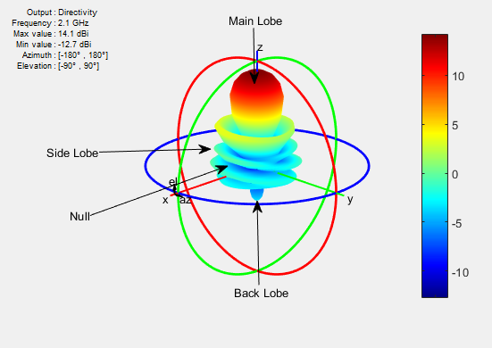
The radiation pattern of an antenna is the spatial distribution of power. The pattern displays the directivity or gain of the antenna. the power pattern of an antenna plots the transmitted or received power for a given radius. The field pattern of an antenna plots the variation in the electric or magnetic field for a given radius. The radiation pattern provides details such as the maximum and minimum value of the field quantity and the range of angles over which data is plotted.

h = helix;
h.Turns = 13;
h.Radius = 0.025;
pattern(h,2.1e9)

Use the pattern function to plot radiation pattern of any antenna in the Antenna Toolbox™. By default, the function plots the directivity of the antenna. You can also plot the electric field and power pattern by using Type name-value pair argument of the pattern function.

Lobes

Each radiation pattern of an antenna contains radiation lobes. The lobes are divided into major lobes (also called main lobes) and minor lobes. Side lobes and back lobes are variations of minor lobes.

h = helix;
h.Turns = 13;
h.Radius = 0.025;
patternElevation(h,2.1e9)

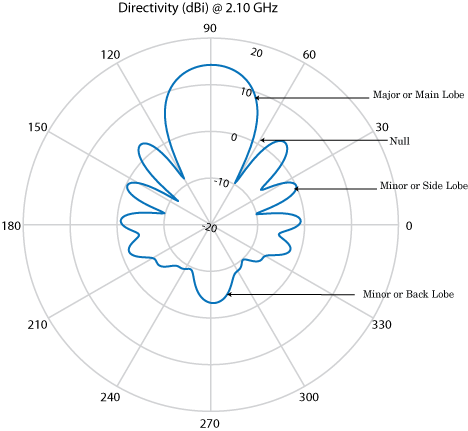
Major or Main lobe: Shows the direction of maximum radiation, or power, of the antenna.
Minor lobe: Shows the radiation in undesired directions of antenna. The fewer the number of minor lobes, the greater the efficiency of the antenna. Side lobes are minor lobes that lie next to the major lobe. Back lobes are minor lobes that lie opposite to the major lobe of antenna.
Null: Shows the direction of zero radiation intensity of the antenna. Nulls usually lie between the major and minor lobe or in between the minor lobes of the antennas.

Field Regions

For an antenna engineer and an electromagnetic compatibility (EMC) engineer, it is important to understand the regions around the antenna.

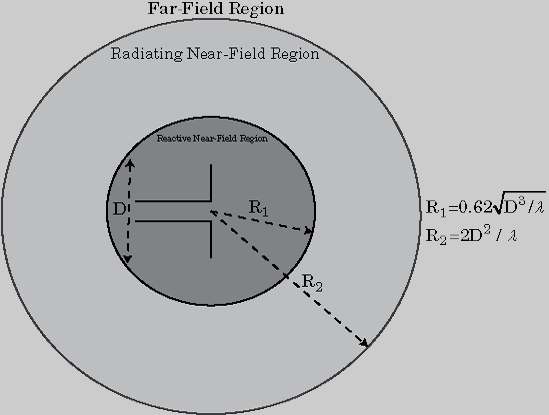
The region around an antenna is defined in many ways. The most used description is a 2- or 3-region model. The 2-region model uses the terms near field and the far field to identify specific dominant field mechanisms. The diagram is a representation of antenna fields and boundaries. The 3-field region splits the near field into a transition zone, where a weakly radiative mechanism is at work.

Near-Field Region: The near-field region is divided into two transition zones: a reactive zone and radiating zone.

Reactive Near-Field Region: This region is closest to the antenna surface. The reactive field dominates this region. The reactive field is stored energy, or standing waves. The fields in this region change rapidly with distance from the antenna. The equation for outer boundary of this region is: $R < 0.62 \sqrt{D^{3} / λ}$ where R is the distance from the antenna, λ is the wavelength, and D is the largest dimension of the antenna. This equation holds true for most antennas. In a very short dipole, the outer boundary of this region is $λ / 2 π$ from the antenna surface.
Radiating Near-Field Region: This region is also called the Fresnel region and lies between the reactive near-field region and the far-field region. The existence of this region depends on the largest dimension of the antenna and the wavelength of operation. The radiating fields are dominant in this region. The equation for the inner boundary of the region is equation $R \geq 0.62 \sqrt{D^{3} / λ}$ and the outer boundary is $R < 2 D^{2} / λ$ . This holds true for most antennas. The field distribution depends on the distance from the antenna.

Far-field Region: This region is also called Fraunhofer region. In this region, the field distribution does not depend on the distance from the antenna. The electric and magnetic fields in this region are orthogonal to each other. This region contains propagating waves. The equation for the inner boundary of the far-field is $R = 2 D^{2} / λ$ and the equation for the outer boundary is infinity.

Directivity and Gain

Directivity is the ability of an antenna to radiate power in a particular direction. It can be defined as ratio of maximum radiation intensity in the desired direction to the average radiation intensity in all other directions. The equation for directivity is:

$D = \frac{4 π U (θ, ϕ)}{P_{r a d}}$

where:

D is the directivity of the antenna
U is the radiation intensity of the antenna
P_rad is the average radiated power of antenna in all other directions

Antenna directivity is dimensionless and is calculated in decibels compared to the isotropic radiator (dBi).

The gain of an antenna depends on the directivity and efficiency of the antenna. It can be defined as the ratio of maximum radiation intensity in the desired direction to the total power input of the antenna. The equation for gain of an antenna is:

$G = \frac{4 π U (θ, ϕ)}{P_{i n}}$

where:

G is the gain of the antenna
U is the radiation intensity of the antenna
P_in is the total power input to the antenna

If the efficiency of the antenna in the desired direction is 100%, then the total power input to the antenna is equal to the total power radiated by the antenna, that is, $P_{i n} = P_{r a d}$ . In this case, the antenna directivity is equal to the antenna gain.

Beamwidth

Antenna beamwidth is the angular measure of the antenna pattern coverage. As seen in the figure, the main beam is a region around maximum radiation. This beam is also called the major lobe, or main lobe of the antenna.

Half power beamwidth (HPBW) is the angular separation in which the magnitude of the radiation pattern decreases by 50% (or -3dB) from the peak of the main beam

Use the beamwidth function to calculate the beamwidth of any antenna in Antenna Toolbox.

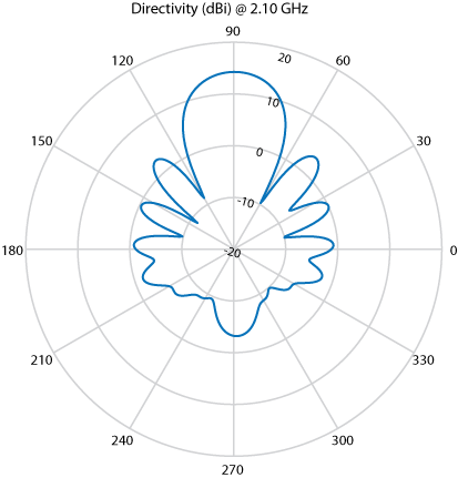
E-Plane and H-Plane

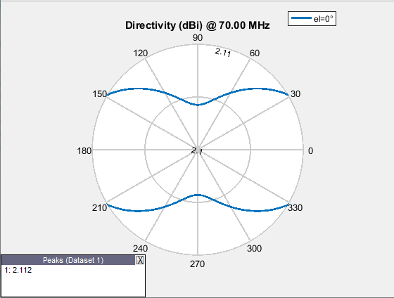
E-plane: Plane containing the electric field vector and the direction of maximum radiation. Consider a dipole antenna that is vertical along the z-axis. Use the patternElevation function to plot the elevation plane pattern. The elevation plane pattern shown captures the E-plane behavior of the dipole antenna.

d = dipole;
patternElevation(d,70e6)

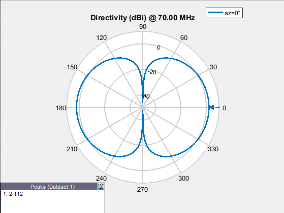
H-plane: Plane containing the magnetic field vector and the direction of maximum radiation. Use the patternAzimuth function to plot the azimuth plane pattern of a dipole antenna. The azimuthal variation in pattern shown captures the H-plane behavior of the dipole antenna.

d = dipole;
patternAzimuth(d,70e6)

Use EHfields to measure the electric and magnetic fields of the antenna. The function can be used to calculate both near and far fields.

Polarization

Polarization is the orientation of the electric field, or E-field, of an antenna. Polarization is classified as elliptical, linear, or circular.

Elliptical polarization: If the electric field remains constant along the length but traces an ellipse as it moves forward, the field is elliptically polarized. Linear and circular polarizations are special cases of elliptical polarization.

Linear polarization: If the electric field vector at a point in space is directed along a straight line, the field is linearly polarized. A linearly polarized antenna radiates only one plane and this plane contains the direction of propagation of the radio waves. There are two types of linear polarization:

Horizontal Polarization: The electric field vector is parallel to the ground plane. To view the horizontal polarization pattern of an antenna, use the pattern function, with the 'Polarization' name-value pair argument set to 'H'. The plot shows the horizontal polarization pattern of a dipole antenna:
```
d = dipole;
pattern(d,70e6,Polarization="H")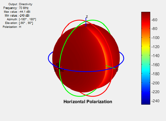
```
USA television networks use horizontally polarized antennas for broadcasting.
Vertical Polarization: The electric field vector is perpendicular to the ground plane. To view the vertical polarization pattern of an antenna, use the pattern function, with the 'Polarization' name-value pair argument set to 'V'. Vertical polarization is used when a signal has to be radiated in all directions. The plot shows the vertical polarization pattern of a dipole antenna:
```
d = dipole;
pattern(d,70e6,Polarization="V")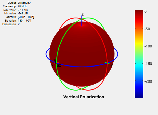
```
An AM radio broadcast antenna or an automobile whip antenna are some examples of vertically polarized antennas.

Circular Polarization: If the electric field remains constant along the straight line but traces circle as it moves forward, the field is circularly polarized. This wave radiates in both vertical and horizontal planes. Circular polarization is most often used in satellite communications. There are two types of circular polarization:

Right-Hand Circularly Polarized (RHCP): The electric field vector is traced in the counterclockwise direction. To view the RHCP pattern of an antenna, use the pattern function, with the 'Polarization' name-value pair argument set to 'RHCP'. The plot shows RHCP pattern of helix antenna:
```
 h = helix;
 h.Turns = 13;
 h.Radius = 0.025;
 pattern(h,1.8e9,Polarization="RHCP")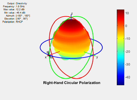
```
Left-Hand circularly polarized (LHCP): The electric field vector is traced in the clockwise direction. To view the LHCP pattern of an antenna, use the pattern function, with the 'Polarization' name-value pair argument set to 'LHCP'. The plot shows LHCP pattern of helix antenna:
```
 h = helix;
 h.Turns = 13;
 h.Radius = 0.025;
 pattern(h,1.8e9,Polarization="LHCP")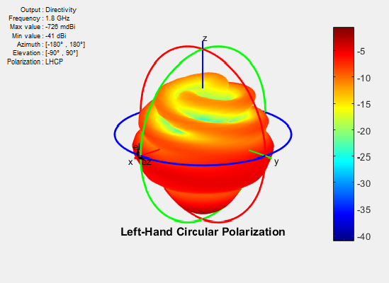
```

For efficient communications, the antennas at the transmitting and receiving end must have same polarization.

Axial Ratio

Axial ratio (AR) of an antenna in a given direction quantifies the ratio of orthogonal field components radiated in a circularly polarized wave. An axial ratio of infinity implies a linearly polarized wave. When the axial ratio is 1, the radiated wave has pure circular polarization. Values greater than 1 imply elliptically polarized waves.

Use axialRatio to calculate the axial ratio for any antenna in the Antenna Toolbox.

References

[1] Balanis, C.A. Antenna Theory. Analysis and Design, 3rd Ed. New York: Wiley, 2005.

[2] Stutzman, Warren.L and Thiele, Gary A. Antenna Theory and Design, 3rd Ed. New York: Wiley, 2013.

[3] Capps, C. Near Field or Far Field, EDN, August 16, 2001, pp.95 - pp.102.