optimize

Optimize antenna and array catalog elements using SADEA or TR-SADEA algorithm

Since R2020b

Syntax

optimizedelement = optimize(element,frequency,objectivefunction,propertynames,bounds)

optimizedelement = optimize(___,Name=Value)

Description

optimizedelement = optimize(element,frequency,objectivefunction,propertynames,bounds) optimizes the antenna or the array at the specified frequency using the specified objective function and the antenna or array properties and their bounds.

optimizedelement = optimize(___,Name=Value) optimizes the antenna or the array using additional options specified by one or more name-value arguments.

Examples

Maximize Gain of Dipole Antenna

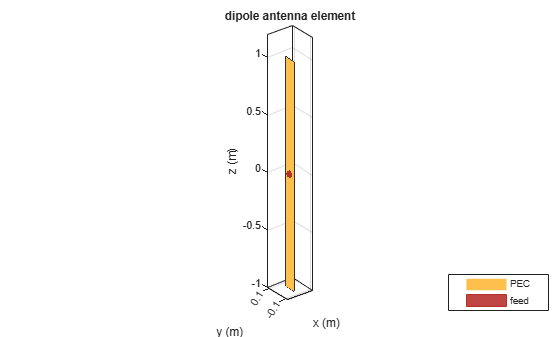
Create and view a default dipole antenna.

ant = dipole;
show(ant)

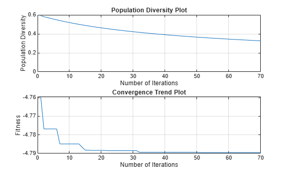
Maximize the gain of the antenna by changing the antenna length from 3 m to 7 m and the width from 0.11 m to 0.13 m.

Optimize the antenna at a frequency of 75 MHz.

optAnt = optimize(ant,75e6,"maximizeGain", ...
                {'Length','Width'}, {3 0.11; 7 0.13})

optAnt = 
  dipole with properties:

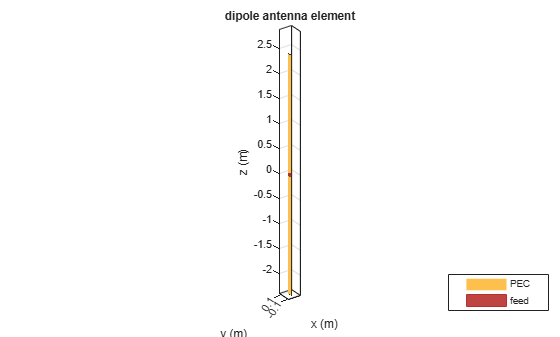
        Length: 4.7979
         Width: 0.1100
    FeedOffset: 0
     Conductor: [1×1 metal]
          Tilt: 0
      TiltAxis: [1 0 0]
          Load: [1×1 lumpedElement]

show(optAnt)            

Optimize E-Notch Microstrip Patch Antenna for Gain with Geometric Constraints

This example shows how to optimize an E-Notch microstrip patch antenna for gain with constraints on its geometry.

Create E-Notch Microstrip Patch Antenna

Create an E-Notch microstrip patch antenna operating at 2GHz and vary its center arm notch length and width.

% Create E-notch microstrip antenna
ant = design(patchMicrostripEnotch,2e9);
ant.CenterArmNotchLength = 0.0073;
ant.CenterArmNotchWidth = 0.0144;

Plot its radiation pattern and check the maximum gain value.

% Check the gain
figure
pattern(ant,2e9,Type="gain")

Optimize E-Notch Microstrip Patch Antenna for Gain

Define the design variables, and their lower and upper bounds.

designVariables = {'CenterArmNotchLength','NotchLength','Width','CenterArmNotchWidth','NotchWidth'};
XVmin = [0.001, 0.03, 0.03, 0.01, 0.001];
XVmax = [0.02, 0.06, 0.07, 0.03, 0.009];

Add geometric constraints

Prepare coefficients in the form of a matrix with reference to below linear inequalities:

1. $$5*\mathrm{CenterArmNotchLength}<\mathrm{NotchLength}$$

2. $$\mathrm{CenterArmNotchWidth}+(2*\mathrm{Notchwidth})<\mathrm{Width}$$

Rewrite the inequalities 1 & 2 in the form of $\mathrm{ax}+\mathrm{by}+\mathrm{cz}\le 0$

1. $$5*\mathrm{CenterArmNotchLength}-\mathrm{NotchLength}<0$$

2. $$\mathrm{CenterArmNotchWidth}+(2*\mathrm{Notchwidth})-\mathrm{Width}<0$$

Convert these inequalities to a matrix of form $\mathrm{AX}<=b$, where $\mathit{A}$ is coefficient matrix and $\mathit{b}$ is constant matrix. Write the coefficients as per the order of design variables.

A = [5,-1,0,0,0;...
     0,0,-1,1,2];

b = [0;0];

Define a structure to contain both the coefficient and constant matrices.

constraintsStructure.A = A;
constraintsStructure.b = b;

Optimize E-Notch microstrip patch antenna and check its gain

Run the optimization on E-Notch microstrip patch antenna leveraging these constraints. Visualize the optimized design and plot the radiation pattern.

optAnt = optimize(ant, 2e9, "maximizeGain", designVariables, {XVmin;XVmax}, Iterations=50, GeometricConstraints=constraintsStructure);

figure
show(optAnt)

figure
pattern(optAnt,2e9,Type="gain")

Input Arguments

element — Antenna or array to optimize

antenna object | array object | customAntenna object

Antenna or array to optimize, specified as an antenna object from the antenna catalog, array object from the array catalog, or customAntenna object.

Note

To optimize pcbStack antenna, use PCB Antenna Designer app.

Example: dipole

Example: linearArray(Element=dipole)

Example: customAntenna(Shape=shape.Rectangle)

frequency — Frequency to optimize antenna or array

positive scalar

Operating frequency of the antenna or array to optimize, specified as a positive scalar in Hertz.

Example: 70e6

Data Types: double

objectivefunction — Objective of antenna or array optimization

"maximizeGain" | "fronttoBackLobeRatio" | "maximizeBandwidth" | "minimizeBandwidth" | "maximizeSLL" | "minimizeArea" | custom objective function | anonymous function handle

Objective of antenna or array optimization, specified as a string from one of the following:

• maximizeGain — Maximize the gain of the given antenna or array element

• fronttoBackRatio — Increase the front-lobe-to-back-lobe ratio of the antenna or array element

• maximizeBandwidth — Maximize the operation bandwidth of the antenna or array element. Use this objective function for optimizing antennas or arrays for wideband applications.

• minimizeBandwidth — Minimize the operation bandwidth of the antenna or array element. Use this objective function for optimizing antennas or arrays for narrowband applications.

• maximizeSLL — Maximize the ratio between the front lobe and the first side lobes of the antenna or array pattern.

• minimizeArea — Minimizes the maximum area occupied by the antenna or the array element. If the dimension of the element in the array is smaller than the aperture, the objective function minimizes the array aperture.

• Custom objective function — Optimizes the antenna or array as per the user defined objective function.

• Anonymous function handle — Optimizes the antenna or array for the objectives defined using the anonymous function handle.

Data Types: string

propertynames — Properties of antenna or array

cell array of character vectors

Properties of the antenna or array object to optimize, specified as a cell array of character vectors. The property names are selected as the design variables in optimization.

Example: {'Length','Width'}

Data Types: cell

bounds — Lower and upper bounds of design variables

two-row cell array

Lower and upper bounds of design variables, specified as a two-row cell array.

Example: {3 0.11; 7 0.13}

Data Types: double

Name-Value Arguments

Specify optional pairs of arguments as Name1=Value1,...,NameN=ValueN, where Name is the argument name and Value is the corresponding value. Name-value arguments must appear after other arguments, but the order of the pairs does not matter.

Example: Constraints={'Area < 0.03'}

Constraints — Optimization constraints

cell array of strings or character vectors

Optimization constraints, specified as a cell array of strings or character vectors. Each character vector or string must be specified in the following format: (analysis function) (inequality sign) (value). You can specify any of the following analysis functions:

• Area in meter square

• Volume in meter cube

• S11 in dB

• Gain in dBi

• F/B in dBi

• SLL in dBi

The inequality signs '<' or '>' and the values specifies the analysis function limits. For example, 'Area < 0.03' indicates that the area of the optimizing antenna must be less than 0.03 square meter.

Example: {'Area < 0.03'}

Data Types: char | string

Weights — Weight or penalty of each constraint function

vector of positive integers in the range (1,100)

Weight or penalty of each constraint function, specified as a vector of positive integers in the range (1,100). If the penalty is set to high, a higher priority is given to the constraint function in case of multiple constraint optimization. All constraint functions are weighted equally by default.

Example: 8

Data Types: double

FrequencyRange — Range of frequencies for vector frequency analysis

vector of positive numbers

Range of frequencies for vector frequency analysis like S-parameters, specified as a vector of positive numbers with each element unit in Hertz.

The default frequency range is obtained from the center frequency considering a bandwidth of less than 10 percent.

Example: linspace(1e9,2e9,10)

Data Types: double

ReferenceImpedance — Reference impedance of optimizing antenna or array

50 (default) | scalar

Reference impedance of antenna or array being optimized, specified as a scalar in ohms.

Example: 75

Data Types: double

MainLobeDirection — Azimuth and elevation of main lobe

[0,90] (default) | two-element vector

Azimuth and elevation of main lobe of antenna or array being optimized, specified as a two-element vector with each element unit in degrees. The first element represents azimuth and the second element represents elevation.

Example: [20 30]

Data Types: double

Iterations — Number of iterations to run optimizer

200 (default) | positive scalar

Number of iterations to run the optimizer after you build the model, specified as a positive scalar.

Example: 40

Data Types: double

UseParallel — Option to enable parallel pool

false (default) | true

Option to enable parallel pool, specified as a logical value. The default value is false. Set this option to true to enable the parallel pool. Use parallel pool to speed up the optimization for computationally large antennas and arrays. To use this feature, you need a license to the Parallel Computing Toolbox™.

Use the canUseParallelPool function to check if Parallel Computing Toolbox is installed and licensed for use, a default parallel pool is configured and supported, and automatic creation of parallel pools is enabled.

Example: true

Data Types: logical

EnableCoupling — Option to enable mutual coupling of elements in arrays during optimization

true (default) | false

Option to enable mutual coupling of elements in an array during optimization, specified as a logical true to enable or false to disable. By default, this option is enabled.

Example: false

Data Types: logical

EnableLog — Option to print iteration number and value of convergence on command line

false (default) | true

Option to print iteration number and value of convergence on the command line, specified as a logical true to enable or false to disable. By default, this option is disabled.

Example: true

Data Types: logical

GeometricConstraints — Geometric constraints

structure

Geometric constraints for optimization, specified as a structure of coefficient matrix and constant vector.

Specify linear inequality constraints in the A matrix and b vector.

• A is a real M-by-N matrix where M is the number of inequalities, and N is the number of design variables. A holds the design variable coefficients of the inequalities.

• b is a real M-element column vector and holds the constants of inequalities corresponding to the coefficients in A.

For example, consider an optimization problem consisting of 5 design variables as follows:

designVariables = {'CenterArmNotchLength','NotchLength','Width',...
            'CenterArmNotchWidth','NotchWidth'};

The geometric constraints for optimization are:

• 5*CenterArmNotchLength - NotchLength < 0

• CenterArmNotchWidth + 2*Notchwidth - Width < 0

Define the A and b as follows:

A = [5,-1,0,0,0;...
     0,0,-1,1,2];
b = [0;0];

Specify linear equality constraints in the Aeq matrix and beq vector.

• Aeq is an Me-by-N matrix, where Me is the number of equalities, and N is the number of design variables. Aeq holds the design variable coefficients of the equalities.

• beq is a real Me-element column vector and holds the constants of equalities corresponding to the coefficients in Aeq.

Specify non-linear inequality constraints in the nlcon matrix and nrlv vector.

• nlcon is a function handle that defines nonlinear constraints. It stores the design variables.

• nrlv is a 1-by-N vector of 0 and 1. N is the number of design variables in nlcon. Each index in nrlv corresponds to a design variable in nlcon in that sequence. Specify 1 at an index in nrlv to convey the optimize function that the corresponding design variable is relevant for optimization. Specify 0 at an index in nrlv to convey the optimize function that the corresponding design variable is not relevant for optimization.

For example, to maximize the gain of a dipole antenna operating at 75 MHz with constraints on its length and width, use this code:

optAnt = optimize(dipole, 75e6, "maximizeGain", {"Length", "Width"},... 
  {LowerBound; UpperBound}, Iterations=150, GeometricConstraints=opt);
opt = 

  struct with fields:

        A: [100×2 double]
        b: [100×1 double]
      Aeq: [-1 5]
      beq: 0
    nlcon: @btw
     nrlv: [1 1]

For additional information on linear and nonlinear equalities and nonlinear inequalities, see the fmincon (Optimization Toolbox) function documentation.

Example: A=[5,-1,0,0,0; 0,0,-1,1,2]; b=[0;0]; structure.A=A; structure.b=b;

Example: Aeq=[-1 5]; beq=0; structure.Aeq=Aeq; structure.beq=beq;

Example: nlcon=@btw; nrlv=[1 1]; structure.nlcon=nlcon; structure.nrlv=nrlv;

Data Types: struct

UseAlgorithm — Algorithm to use for antenna or array optimization

"SADEA" (default) | "TR-SADEA"

Algorithm to use for antenna or array optimization, specified as a string. By default, the optimize function uses SADEA algorithm. Use TR-SADEA for applications where the evaluation of the objective function is computationally expensive. For more information, see optimization algorithms.

Example: UseAlgorithm="TR-SADEA"

Data Types: string

Output Arguments

optimizedelement — Optimized antenna or array element

antenna object | array object | customAntenna object

Optimized antenna or array element, returned as an antenna, array, or customAntenna object.

Version History

Introduced in R2020b

R2024b: New features

The optimize function has added three new features:

Support for custom geometric constraints defined using linear equalities and nonlinear inequalities

You can now use custom geometric constraints defined by linear equalities and nonlinear inequalities for antenna or array optimization. Define the custom geometric constraints in the GeometricConstraints property of the optimize function using the opt structure that contains the coefficients of linear inequalities (A, b) and equalities (Aeq, beq) and nonlinear inequalities (nlcon, nrlv).

Optimize antennas and arrays using Training Cost Reduced SADEA (TR-SADEA) algorithm

Optimize large antennas and arrays using the TR-SADEA algorithm in the optimize function. Set the new UseAlgorithm argument in the optimize function to "TR-SADEA" to use TR-SADEA algorithm for your optimization task. To use this feature, you need a license for Statistics and Machine Learning Toolbox™ in addition to Antenna Toolbox™.

Support for anonymous function handle in optimization

You can now use an anonymous function handle to define antenna or array optimization objectives in the optimize function.

R2024a: Use custom objective function and geometric constraints for optimization

• Specify a custom objective function to define antenna or array optimization objectives.

• Use custom geometric constraints defined by linear inequalities of design variables for antenna or array optimization. Specify custom geometric constraints in the new GeometricConstraints name-value argument.