Detect and Track LEO Satellite Constellation with Ground Radars
R2026bThis example shows how to import a Two-Line Element (TLE) file of a satellite constellation, simulate radar detections of the constellation, and track the constellation.
The task of populating and maintaining a catalog of space objects orbiting Earth is crucial in space surveillance. This task consists of several processes: detecting and identifying new objects and adding them to the catalog, updating known object orbits in the catalog, tracking orbit changes throughout their lifetime, and predicting reentries in the atmosphere. In this example, we study how to detect and track new satellites and add them to a catalog.
To guarantee safe operations in space and prevent collisions with other satellites or known debris, it is important to correctly detect and track newly launched satellites. Space agencies typically share prelaunch information, which can be used to select a search strategy. A Low Earth Orbit (LEO) satellite search strategy consisting of fence-type radar systems is commonly used. A fence-type radar system searches a finite volume in space and detects satellites as they pass through its field of view. This strategy can detect and track a newly launched constellation quickly [1].
Import Satellite Constellation from TLE File
Two-Line Element sets are a common data format to save orbital information of satellites. You can use the satelliteScenario object to import satellite orbits defined in a TLE file. By default, the imported satellite orbits are propagated using the SGP4 orbit propagation algorithm which provides good accuracy for LEO objects. In this example, these orbits provide the ground truth to test the radar tracking system capability to detect newly launched satellites.
rng(2020); % For repeatable results
% Create a satellite scenario
satscene = satelliteScenario;
% Add satellites from TLE file.
tleFile = "leoSatelliteConstellation.tle";
constellation = satellite(satscene, tleFile);
numSatellites = numel(constellation);
initialUTC = satscene.StartTime; % Start time derived from TLE file
Use the satellite scenario viewer to visualize the constellation.
play(satscene);
Model Space Surveillance Radars
Define two stations with fan-shaped radar beams looking into space. The fans cut through the satellite orbits to maximize the number of detections. The radar stations located on North America form an East-West fence.
% First station coordinates in LLA
station1LLA = [48 -76 0];
% Second station coordinates in LLA
station2LLA = [50 -117 0];
Each station is equipped with a radar, which is modeled by using a fusionRadarSensor object. In order to detect satellites in the LEO range, the radar has the following requirements:
Detecting a 10 dBsm object up to 2000 km away
Resolving objects horizontally and vertically with a precision of 100 m at 2000 km range
Having a field of view of 120 degrees in azimuth and 40 degrees in elevation
Looking up into space
Reporting measurements in azimuth, elevation, range, and range-rate
% Create fan-shaped monostatic radars
fov = [120;40];
updateRate = 0.5; % Hz
radar1 = fusionRadarSensor(1,...
    UpdateRate=updateRate,...
    ScanMode="No scanning",...
    MountingAngles=[0 90 0],... % Look up
    FieldOfView=fov,... % degrees
    ReferenceRange=2000e3,... % m
    RangeLimits=[0 2000e3],... % m
    RangeRateLimits=[-1e5 1e5],... % m/s
    ReferenceRCS=10,... % dBsm
    HasFalseAlarms=false,...
    HasNoise=true,...
    HasElevation=true,...
    HasRangeRate=true,...
    AzimuthResolution=0.03,... % degrees
    ElevationResolution=0.03,... % degrees
    RangeResolution=2000,... % m
    RangeRateResolution=400,... % m/s
    DetectionCoordinates="Sensor Spherical",...
    TargetReportFormat="Detections");

radar2 = clone(radar1);
radar2.SensorIndex = 2;
Radar Processing Chain
In this example, a few coordinate transformations are performed to properly run the radar tracking chain. The diagram below illustrates how the inputs are transformed and passed to the radar and used to generate detection data.
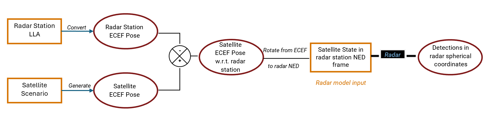
In the first step, you calculate satellite poses expressed in the North-East-Down (NED) frame of each radar station as shown above. You achieve this by first obtaining the poses of the satellites with respect to the radar station in the Earth-Centered-Earth-Fixed (ECEF) frame and then transforming them to the radar station's NED frame. See the assembleRadarInputs supporting function for the implementation details. Next, you use the simulated fusionRadarSensor to generate detections based on the NED poses.
Define Tracker
To estimate the satellite orbits based on the detections reported by the radar, you use a tracker. The Sensor Fusion and Tracking Toolbox™ provides a variety of multi-object trackers. In this example, you choose a task-oriented global nearest neighbor (GNN) tracker. In a task-oriented tracking workflow, you first define the specifications of the targets and the specifications of the sensors. You then use these specifications to define the tracker.
Specify Target Type
In this step, you specify the type and the characteristics of the objects you intend to track. You use the trackerTargetSpec function to create a target spec that models Keplerian motion as follows.
satelliteSpec = trackerTargetSpec("space","earth-centered","keplerian");
disp(satelliteSpec)
  EarthCenteredKeplerian with properties:

                   MinAltitude: 1.2e+05    m
                   MaxAltitude: 2e+06      m
                      MaxSpeed: 8000       m/s
    MaxDisturbanceAcceleration: 0.02       m/s²
The display above shows the list of properties of the Keplerian target specification, which can be modified for your application. The specification models target states as in the Earth-Centered Inertial (ECI) frame. The MinAltitude and MaxAltitude properties specify the region of interest for tracking. The MaxSpeed property sets the upper limit for the magnitude of a target’s initial velocity. The MaxDisturbanceAcceleration property defines the extent of motion uncertainty, accounting for unmodeled perturbations such as higher-order gravitational effects, atmospheric drag, and solar radiation pressure.
Note that the target specification uses a Keplerian motion model to propagate satellite motion, which has lower fidelity than SGP4. In practice, this modeling inaccuracy is typically mitigated through measurement updates and the inclusion of process noise, represented by the MaxDisturbanceAcceleration parameter in the target specification.
Specify Sensor Type
After specifying the objects to track, you specify the sensors you use for tracking. Use the trackerSensorSpec function to create the ground radar specification for the first radar.
radarSpec1 = trackerSensorSpec("space","ground-based","radar")
radarSpec1 =
  SpaceGroundBasedRadar with properties:

           MaxNumLooksPerUpdate: 30
    MaxNumMeasurementsPerUpdate: 10

              ReferenceFrame: 'NED'
       GroundStationPosition: [0 0 0]         [deg deg m]
    GroundStationOrientation: [3⨯3 double]
            MountingLocation: [0 0 0]         m
              MountingAngles: [0 0 0]         deg

       HasElevation: 1
       HasRangeRate: 1
        FieldOfView: [60 20]           deg
        RangeLimits: [1e+05 2e+06]     m
    RangeRateLimits: [-10000 10000]    m/s

      AzimuthResolution: 1      deg
        RangeResolution: 100    m
    ElevationResolution: 5      deg
    RangeRateResolution: 10     m/s

    DetectionProbability: 0.9
          FalseAlarmRate: 1e-06

    Terrain: 'none'
Then, specify the characteristics of the sensor spec based on the sensors you simulated in the last section.
radarSpec1.GroundStationPosition = station1LLA;
radarSpec1.MountingAngles =[0 90 0];
radarSpec1.HasRangeRate = true;
radarSpec1.FieldOfView = fov;
radarSpec1.AzimuthResolution = 0.03;
radarSpec1.ElevationResolution = 0.03;
radarSpec1.RangeResolution = 2000;
radarSpec1.RangeRateResolution = 400;
radarSpec1.DetectionProbability = 0.9;
% radarSpec1.FalseAlarmRate = 1e-40;
radarSpec1.RangeLimits = [0 2e6];
radarSpec1.RangeRateLimits = [-1e5 1e5];
The second sensor only differs from the first sensor by its station position. Therefore, you create a copy of the first sensor spec and modify its station position.
radarSpec2 = radarSpec1;
radarSpec2.GroundStationPosition = station2LLA;
Configure Tracker
In this step, you create a tracker based on the created target spec and sensor specs. As mentioned, you use the GNN algorithm.
tracker = multiSensorTargetTracker(satelliteSpec,{radarSpec1,radarSpec2},"gnn");With this simple setup, the tracker configures the right motion model. Also, the tracker configures the right observability, measurement, clutter, birth, and state initialization models automatically.
disp(tracker)
  fusion.tracker.GNNHistoryTracker with properties:

         TargetSpecifications: {[1×1 EarthCenteredKeplerian]}
         SensorSpecifications: {[1×1 SpaceGroundBasedRadar]  [1×1 SpaceGroundBasedRadar]}
       MaxMahalanobisDistance: 5
    NumUpdatesForConfirmation: [2 3]
         NumMissesForDeletion: [5 5]
You can tune the tracker by changing the MaxMahalanobisDistance, NumUpdatesForConfirmation, and NumMissesForDeletion properties.
Sensor Data Format
The sensor specifications define the format of the data that the tracker expects. You can view this format using the dataFormat object function.
format = dataFormat(radarSpec1)
format = struct with fields:
             LookTime: [01-Jan-1970    01-Jan-1970    01-Jan-1970    01-Jan-1970    01-Jan-1970    01-Jan-1970    01-Jan-1970    01-Jan-1970    01-Jan-1970    01-Jan-1970    01-Jan-1970    01-Jan-1970    01-Jan-1970    …    ] (1×30 datetime)
          LookAzimuth: [0 0 0 0 0 0 0 0 0 0 0 0 0 0 0 0 0 0 0 0 0 0 0 0 0 0 0 0 0 0]
        LookElevation: [0 0 0 0 0 0 0 0 0 0 0 0 0 0 0 0 0 0 0 0 0 0 0 0 0 0 0 0 0 0]
        DetectionTime: [01-Jan-1970    01-Jan-1970    01-Jan-1970    01-Jan-1970    01-Jan-1970    01-Jan-1970    01-Jan-1970    01-Jan-1970    01-Jan-1970    01-Jan-1970]
              Azimuth: [0 0 0 0 0 0 0 0 0 0]
            Elevation: [0 0 0 0 0 0 0 0 0 0]
                Range: [0 0 0 0 0 0 0 0 0 0]
            RangeRate: [0 0 0 0 0 0 0 0 0 0]
      AzimuthAccuracy: [0 0 0 0 0 0 0 0 0 0]
    ElevationAccuracy: [0 0 0 0 0 0 0 0 0 0]
        RangeAccuracy: [0 0 0 0 0 0 0 0 0 0]
    RangeRateAccuracy: [0 0 0 0 0 0 0 0 0 0]
The data format captures everything you need to provide for sensor scanning and measurements. It includes fields to specify the sensor's scanning information as well as measurement information. Each of these fields is populated with nominal values to match the MaxNumLooksPerUpdate and MaxNumMeasurementsPerUpdate values set in the sensor specification. In the next section, you use the supporting function, helperGenerateSensorData, to generate sensor data following this required format.
Simulate Synthetic Detections and Track Constellation
Generate Satellite Trajectories
You first generate the entire history of the states of the constellation over 3 hours.
satscene.StopTime = satscene.StartTime + hours(3);
satscene.SampleTime = floor(1/updateRate); % seconds
numSteps = ceil(seconds(satscene.StopTime - satscene.StartTime)/satscene.SampleTime);

% Generate satellite ECEF pose for downstream sensor data generation
[posECEF, velECEF, utc] = states(constellation,CoordinateFrame="ecef");
% Generate satellite ECI pose for downstream tracking metrics evaluation
[posECI, velECI] = states(constellation,CoordinateFrame="inertial");
poseStruct = struct(Datetime=datetime.empty(), ...
    PlatformID=0, ...
    Position=[0 0 0], ...
    Velocity=[0 0 0], ...
    PositionECI=[0 0 0], ...
    VelocityECI=[0 0 0]);
plats = repmat(poseStruct, numSteps, numSatellites);

for step=1:numSteps
    for jj = 1:numSatellites
        plats(step,jj).Datetime = utc(step);
        plats(step,jj).PlatformID = jj;
        plats(step,jj).Position = posECEF(:,step,jj)';
        plats(step,jj).Velocity = velECEF(:,step,jj)';
        plats(step,jj).PositionECI = posECI(:,step,jj)';
        plats(step,jj).VelocityECI = velECI(:,step,jj)';
    end
end
Configure Visualization
Next, create a radar plot to compare satellite positions with detections within the radar field of view, and a globe viewer to visualize the relationships among detections, ground truth, and tracks.
% Create radar plots
radarplt = helperRadarPlot(fov);
% Create tracking globe viewer
viewer = trackingGlobeViewer(ShowDroppedTracks=false, ...
    PlatformHistoryDepth=5000, ...
    TrackHistoryDepth=5000, ...
    NumCovarianceSigma=3);
Run Simulation
The following steps are performed iteratively:
Generate radar detections and update the tracker with these detections.
Update the radar plot to compare satellite positions with detections within the radar field of view.
Update the globe viewer to display ground truth, detections, and tracks.
% Reset
release(tracker);
clear(viewer);
trackLog = cell(1,numSteps);
step = 0;

% Simulate tracking loop
while step < numSteps
    time = step*satscene.SampleTime;
    step = step + 1;

    % Generate radar data
    targets1 = assembleRadarInputs(station1LLA, plats(step,:));
    targets2 = assembleRadarInputs(station2LLA, plats(step,:));
    data1 = helperGenerateSensorData(radar1,targets1,initialUTC,time,format);
    data2 = helperGenerateSensorData(radar2,targets2,initialUTC,time,format);

    % Update radar plots
    updateRadarPlots(radarplt,targets1,targets2,data1,data2);

    % Generate and update tracks
    confTracks = tracker(data1,data2);
    trackLog{step} = confTracks;

    % Update globe display
    if step == 1 % Plot sensor coverage once for non-scanning radar
        plotCoverage(viewer,{data1,data2},{radarSpec1,radarSpec2});
    end
    plotPlatform(viewer, plats(step,:),'ECEF', Color=[1 0 0], LineWidth=1);
    plotSensorData(viewer,{data1,data2},{radarSpec1,radarSpec2});
    plotTrack(viewer,confTracks,satelliteSpec, LabelStyle="Custom", ...
        CustomLabel="T" + string([confTracks.TrackID]), ...
        Color=[0 1 0], LineWidth=3);
end
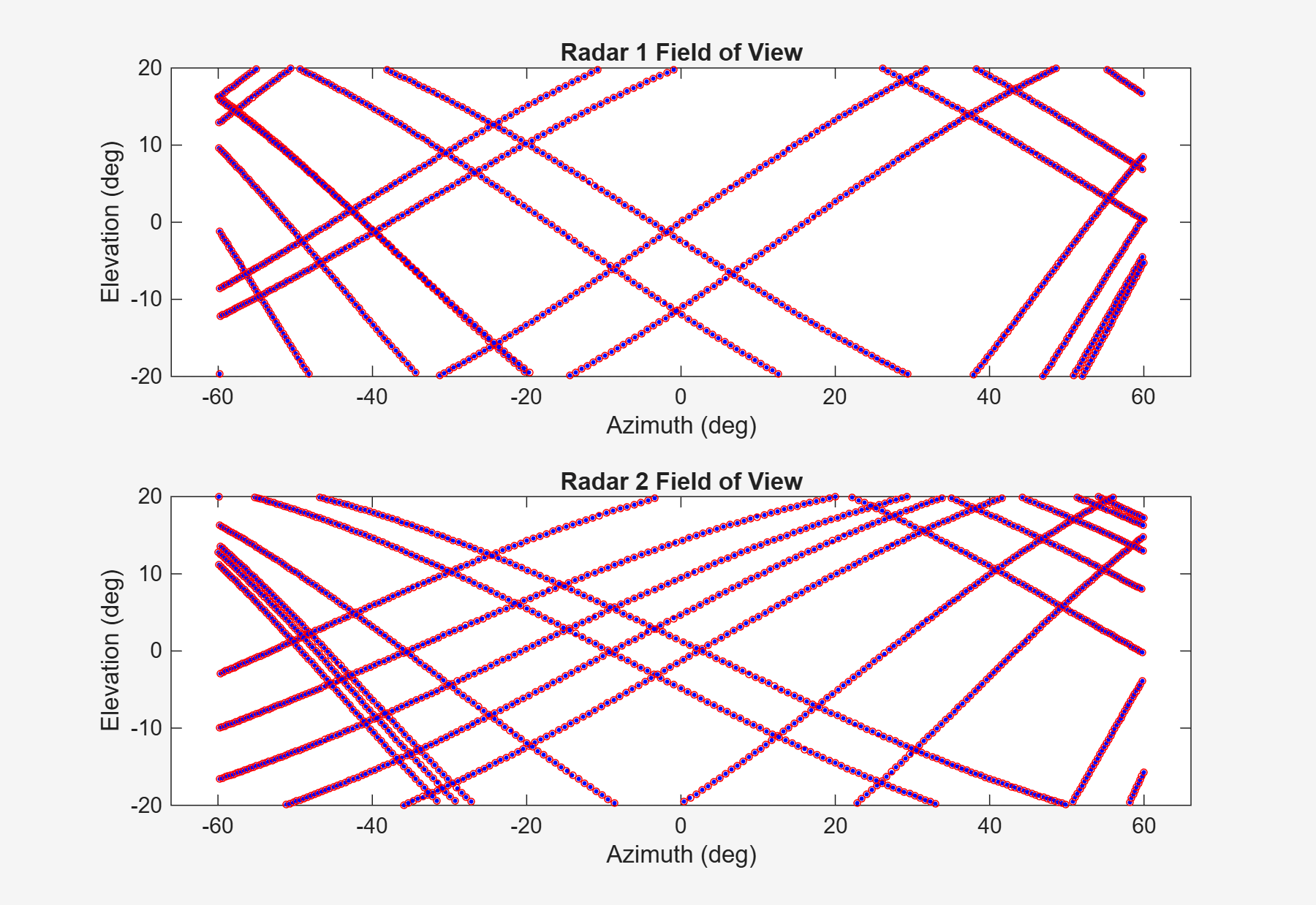
The plot above shows the satellite position (blue dots) and the detections (red circles) from the point of view of each radar.
figure;
snapshot(viewer);
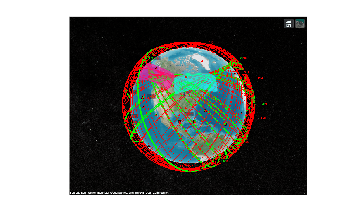
After three hours of tracking, only about half of the constellation is successfully tracked. Maintaining tracks with partial orbit coverage is difficult, as satellites can remain undetected for extended periods in this configuration. In this scenario, only two radar stations are available. Expanding the network with additional stations distributed globally would improve observability and lead to better tracking performance.
Evaluate Track Assignment Metrics
You use assignment metrics to evaluate tracking performance by computing the associations between true objects and tracks.
tam = trackAssignmentMetrics(DistanceFunctionFormat="custom",...
    AssignmentDistanceFcn=@distanceFcn,...
    DivergenceDistanceFcn=@distanceFcn,...
    TruthIdentifierFcn=@(x)[x.PlatformID],...
    AssignmentThreshold=1000,...
    DivergenceThreshold=2000);

for i=1:numSteps
    % Extract the tracker and ground truth at the i-th tracker update
    tracks = trackLog{i};
    truths = plats(i,:);
    % Extract summary of assignment metrics against tracks and truths
    [trackAM,truthAM] = tam(tracks, truths);
end
% Show cumulative metrics for each individual recorded truth object
results = truthMetricsTable(tam);
results(:,{'TruthID','AssociatedTrackID','BreakLength','EstablishmentLength'})
ans = 40×4 table
    TruthID    AssociatedTrackID    BreakLength    EstablishmentLength
    _______    _________________    ___________    ___________________

       1               26                0                1090
       2               20                0                2947
       3               22                0                 285
       4               15                0                2438
       5               28                0                2150
       6               10                0                 969
       7               17                0                2543
       8                2                0                 227
       9              NaN                0                5400
      10               27                0                4427
      11              NaN                0                5400
      12               29                0                5270
      13              NaN                0                5400
      14              NaN                0                5400
      15              NaN                0                5400
      16              NaN                0                5400

	Get insights using Copilot
      ⋮
The table above lists 40 satellites in the launched constellation and shows the tracked satellites with associated track IDs. A track ID of value NaN indicates that the satellite is not tracked by the end of the simulation. This either means that the orbit of the satellite did not pass through the field of view of one of the two radars or the track of the satellite has been dropped. The tracker can drop the track if the satellite is not re-detected soon enough, such that the lack of updates leads to divergence and eventually deletion.
Summary
In this example, you have learned how to use the satelliteScenario object from the Aerospace Toolbox to import orbit information from TLE files. You propagated the satellite trajectories using SGP4 and visualized the scenario using the Satellite Scenario Viewer. You learned how to use the radar and tracker models from the Sensor Fusion and Tracking Toolbox™ to model a space surveillance radar tracking system. The constructed tracking system can predict the estimated orbit of each satellite using a low fidelity model.
Supporting Functions
assembleRadarInputs Derive constellation poses in each radar station frame.
function targetsNED = assembleRadarInputs(station, platsPV)
% For each satellite in the constellation, derive its pose with respect to
% the radar frame.

% Template structure
targetTemplate = struct( ...
    'PlatformID', 0, ...
    'ClassID', 0, ...
    'Position', zeros(1,3), ...
    'Velocity', zeros(1,3), ...
    'Orientation', quaternion(1,0,0,0), ...
    'AngularVelocity', zeros(1,3));

% Pre-compute station pose in ECEF
Recef2station = dcmecef2ned(station(1), station(2));
stationPosECEF = lla2ecef(station);

% Transform all targets from ECEF to NED in a single loop
targetsNED = repmat(targetTemplate, 1, numel(platsPV));
for i = 1:numel(platsPV)
    % Transform position and velocity to NED frame
    targetsNED(i).Position(:) = Recef2station * (platsPV(i).Position(:) - stationPosECEF(:));
    % Simple rotation of target velocity from ECEF to station NED frame
    targetsNED(i).Velocity(:) = Recef2station * platsPV(i).Velocity(:);
    targetsNED(i).PlatformID = platsPV(i).PlatformID;
end
end
helperGenerateSensorData Generate radar detections following the data format required by task-oriented tracker.
function sensorData = helperGenerateSensorData(radar,targets,initialUTC,time,format)
% Generate detections
dets = radar(targets, time);
% Get field names from the format structure
fields = fieldnames(format);
% Initialize each field in the format structure with an empty array
for i = 1:length(fields)
    className = class(format.(fields{i}));
    format.(fields{i}) = feval([className,'.empty'],1,0);
end

sensorData = format;
% Sensor look information
sensorData.LookTime = initialUTC + seconds(time);
sensorData.LookAzimuth = radar.LookAngle(1);
sensorData.LookElevation = radar.LookAngle(2);
sensorData.DetectionTime.TimeZone = "UTC"; % Set time zone for concatenation with UTC datetime.
% Sensor detection information
for ii = 1:numel(dets)
    detection = dets{ii};
    sensorData.DetectionTime = [sensorData.DetectionTime, initialUTC+seconds(detection.Time)];
    sensorData.Azimuth = [sensorData.Azimuth detection.Measurement(1)];
    sensorData.Elevation = [sensorData.Elevation detection.Measurement(2)];
    sensorData.Range = [sensorData.Range detection.Measurement(3)];
    sensorData.RangeRate = [sensorData.RangeRate detection.Measurement(4)];

    azimuthAccuracy = sqrt(detection.MeasurementNoise(1,1));
    elevationAccuracy = sqrt(detection.MeasurementNoise(2,2));
    rangeAccuracy = sqrt(detection.MeasurementNoise(3,3));
    rangeRateAccuracy = sqrt(detection.MeasurementNoise(4,4));
    sensorData.AzimuthAccuracy = [sensorData.AzimuthAccuracy azimuthAccuracy];
    sensorData.ElevationAccuracy = [sensorData.ElevationAccuracy elevationAccuracy];
    sensorData.RangeAccuracy = [sensorData.RangeAccuracy rangeAccuracy];
    sensorData.RangeRateAccuracy = [sensorData.RangeRateAccuracy rangeRateAccuracy];
end
end
distanceFcn Calculate distance for track assignment metric.
function d = distanceFcn(track, truth)
true = [truth.PositionECI(:); truth.VelocityECI(:)];
estimate = track.State([1 3 5 2 4 6]);
cov = track.StateCovariance([1 3 5 2 4 6], [1 3 5 2 4 6]);
d = (estimate - true)' / cov * (estimate - true);
end
Reference
[1] Sridharan, Ramaswamy, and Antonio F. Pensa, eds. Perspectives in Space Surveillance. MIT Press, 2017.

