Orbit Propagation Methods

The Aerospace Blockset™ supports two top-level orbit propagation methods: Kepler (unperturbed) and Numerical (high precision).

Kepler (unperturbed)

Kepler orbit propagation is the process of numerically computing and predicting the position and velocity of an object in space, based on Kepler's laws of planetary motion. Kepler's laws provide a mathematical description of the motion of objects in elliptical orbits around a central body, such as a planet orbiting the Sun.

To propagate a Keplerian orbit, you typically need these elements:

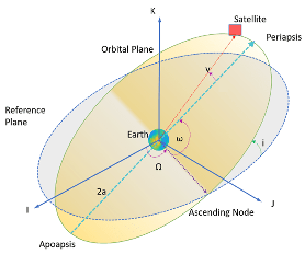
In this diagram, the orbital plane (yellow) intersects a reference plane (gray). For Earth-orbiting satellites, the reference plane is usually the IJ-plane of the GCRF.

These two elements define the shape and size of the ellipse:

• Eccentricity (e) — Describe how elongated the shape of the ellipse is when compared to a circle.

• Semimajor axis (a) — The sum of the periapsis and apoapsis distances divided by 2. Periapsis is the point at which an orbiting object is closest to the center of mass of the body it is orbiting. Apoapsis is the point at which an orbiting object is farthest away from the center of mass of the body it is orbiting. For classic two-body orbits, the semimajor axis is the distance between the centers of the bodies.

These two elements define the orientation of the orbital plane in which the ellipse is embedded:

• Inclination (i) — The vertical tilt of the ellipse with respect to the reference plane measured at the ascending node. The ascending node is the location where the orbit passes upward through the reference plane (the green angle i in the diagram). The tilt angle is measured perpendicular to the line of intersection between orbital plane and the reference plane. Any three points on an ellipse defines the ellipse orbital plane.

  Starting with an equatorial orbit, the orbital plane can be tilted up. The angle it is tilted up from the equator is referred to as the inclination angle, i, in the range [0,180]. Because the center of the Earth must always be in the orbital plane, the point in the orbit where the satellite passes the equator on its way up north-bound through the orbit is the ascending node, and the point where the satellite passes the equator on its way down south-bound is the descending node. Drawing a line through these two points on the equator defines the line of nodes.

• Right ascension of ascending node (Ω) — The horizontal orientation of the ascending node of the ellipse (where the orbit passes upward through the reference plane) with respect to the I-axis of the reference frame. The rotation of the right ascension of the ascending node (RAAN) can be any number between 0° and 360°.

The remaining two elements are:

• Argument of periapsis (ω) — The orientation of the ellipse in the orbital plane, as an angle measured from the ascending node to the periapsis in the range [0, 360).

• True Anomaly (v) — The position of the orbiting body along the ellipse at a specific time. The position of the satellite on the path is measured counterclockwise from the periapsis and is called the true anomaly, ν, in the range [0, 360).

You can propagate the orbit using numerical methods such as numerical integration or Kepler's equation using these parameters. These methods allow you to calculate the position and velocity of the object at a given time. For information on each of these elements, see Orbital Elements.

The Aerospace Blockset uses universal variables and Newton-Raphson iteration to propagate satellite orbits over time. This analytical algorithm is fast, but has limitations. Propagated orbits account only for central body spherical (point-mass) gravity. This formulation includes no other perturbations.

This propagation method is always performed in the ICRF inertial coordinate system with origin at the center of the central body. Given initial inertial position r₀ and velocity v₀ at time t₀, first find orbital energy, ξ, and the reciprocal of the semi-major axis, α:

$\begin{array}{l}\xi =\frac{v_0{}^2}{2}-\frac{\mu }{r_0}\\ \alpha =\frac{-2\xi }{\mu },\end{array}$

where μ is the standard gravitation parameter of the central body. Next, determine the orbit type from the sign of α.

• α>0 => Circular or elliptical

• α<0 => Hyperbolic

• α≈0 => Parabolic

To initialize the Newton-Raphson iteration, select an initial guess for χ based on the orbit type:

• Circular or elliptical orbit

  ${\chi }_0\approx \sqrt{\mu }(\Delta t)\alpha ,$

  where Δt is the propagation step size (simulation time step). If Δt exceeds the orbital period $T=2\pi \sqrt{\frac{a^3}{\mu }}$, wrap Δt.

• Parabolic orbit

  ${\chi }_0\approx \sqrt{p}2\cot (2w),$

  where:

  $\begin{array}{l}\overrightarrow{h}=\overrightarrow{r_0}\times \overrightarrow{v_0}\\ p=\frac{h\cdot h}{\mu }\\ \cot (2s)=3\sqrt{\frac{\mu }{p^3}}(\Delta t)\\ {\tan }^3(w)=\tan (s).\end{array}$

• Hyperbolic orbit:

  ${\chi }_0\approx \text{sign}(\Delta t)\sqrt{-\frac{1}{\alpha }}\ln (\frac{-2\mu \alpha (\Delta t)}{\overrightarrow{r_0}\cdot \overrightarrow{v_0}+\text{sign}(\Delta t)\sqrt{-\frac{\mu }{\alpha }}(1-r_0\alpha )}).$

  Perform Newton-Raphson iteration while |x_n-x_n-1| > tolerance.

  $$\begin{array}{l}{\chi }_{n+\text{1}}={\chi }_n+\frac{\sqrt{\mu }(\Delta t)-{\chi }_n{}^3{c}_3-\frac{\overrightarrow{r_0}\cdot \overrightarrow{v_0}}{\sqrt{\mu }}{\chi }_n{}^2{c}_2-r_0{\chi }_n(1-\psi c_3)}{{\chi }_n{}^2{c}_2+\frac{\overrightarrow{r_0}\cdot \overrightarrow{v_0}}{\sqrt{\mu }}{\chi }_n(1-\psi c_3)+r_0(1-\psi c_2)}\\ {\chi }_n\Leftarrow {\chi }_{n+\text{1}},\end{array}$$

  where:

  $$\psi ={\chi }_n{}^2\alpha .$$

  (if ψ>0),

  $\begin{array}{l}{c}_2=\frac{1-\cos (\sqrt{\psi })}{\psi }\\ c_3=\frac{\sqrt{\psi }-\sin (\sqrt{\psi })}{\sqrt{{\psi }^3}}.\end{array}$

  (if ψ<0),

  $\begin{array}{l}{c}_2=\frac{1-\cosh (\sqrt{-\psi })}{\psi }\\ c_3=\frac{\sinh (\sqrt{-\psi })-\sqrt{-\psi }}{\sqrt{{(-\psi )}^3}}.\end{array}$

  (if ψ≈0),

  $\begin{array}{l}{c}_2=\frac{1}{2}\\ c_3=\frac{1}{6}.\end{array}$

  Calculate universal variables $$f$$, $$\dot{f}$$, $$\text{g}$$, and $$\dot{g}$$.

  $\begin{array}{l}f=1-\frac{{\chi }_n{}^2}{r_0}{c}_2\\ \dot{f}=\frac{\sqrt{\mu }}{r{r}_0}{\chi }_n(\psi c_3-1)\\ g=(\Delta t)-\frac{{\chi }_n{}^3}{\sqrt{\mu }}{c}_3\\ \dot{g}=1-\frac{{\chi }_n{}^2}{r}{c}_2.\end{array}$

  Assemble position and velocity output vectors:

  $\begin{array}{l}\overrightarrow{r_{\text{icrf}}}=f\overrightarrow{r_0}+g\overrightarrow{v_0}\\ \overrightarrow{v_{\text{icrf}}}=\dot{f}\overrightarrow{r_0}+\dot{g}\overrightarrow{v_0}.\end{array}$

Numerical (high precision)

This option uses the Simulink^® solver to integrate position and velocity from central body gravitational acceleration at each simulation timestep (Δt). The method for computing central body acceleration depends on the current setting for the Gravitational potential model parameter. You can also include custom acceleration components in the propagation algorithm using the A_icrf (applied acceleration) input port. For gravity models that include nonspherical acceleration terms, the block computes nonspherical gravity in a fixed-frame coordinate system (ITRF, in the case of Earth). Numerical integration, however, is always performed in the inertial ICRF coordinate system. Therefore, at each timestep:

1. The block transforms position and velocity states into the fixed-frame.

2. The block calculates nonspherical gravity in the fixed-frame.

3. The block transforms resulting acceleration into the inertial frame, where it is summed with the other acceleration terms and integrated.

$\begin{array}{l}\overrightarrow{a_{\text{icrf}}}={\overrightarrow{a}}_{\text{central}\text{body}\text{gravity}}+{\overrightarrow{a}}_{\text{applied}}\\ \overrightarrow{a_{\text{icrf}}}\underset{\text{integrate}}{\Rightarrow }\overrightarrow{r_{\text{icrf}}},\overrightarrow{v_{\text{icrf}}}\end{array}$

Central Body

Methods for computing central body acceleration include point-mass, oblate ellipsoid, or spherical harmonics.

• Point-mass (available for all central bodies) — This option treats the central body as a point-mass, including only the effects of spherical gravity using Newton's law of universal gravitation.

  ${\overrightarrow{a}}_{\text{centralbodygravity}}=-\frac{\mu }{r^2}\frac{\overrightarrow{r_{\text{icrf}}}}{r},$

  where μ is the standard gravitation parameter of the central body.

• Oblate ellipsoid (J2) (available for all central bodies) — In addition to spherical gravity, this option includes the perturbing effects of the second-degree, zonal harmonic gravity coefficient J₂, accounting for the oblateness of the central body. J₂ accounts for the vast majority of the central bodies gravitational departure from a perfect sphere.

  $${\stackrel{\rightharpoonup }{a}}_{centralbodygravity}=-\frac{\mu }{r^2}\frac{\overrightarrow{r_{\text{icrf}}}}{r}+fixed2inertial({\stackrel{\rightharpoonup }{a}}_{nonspherical}),$$

  where:

  $$\begin{array}{l}{\overrightarrow{a}}_{\text{nonspherical}}=\\ \{[\frac{1}{r}\frac{\partial }{\partial r}U-\frac{r_{\text{ff}}{}_{{}_k}}{r^2\sqrt{r_{\text{ff}}{{}_{{}_i}}^2+r_{\text{ff}}{{}_{{}_j}}^2}}\frac{\partial }{\partial \varphi }U]r_{\text{ff}}{}_{{}_i}\}i\\ +\{[\frac{1}{r}\frac{\partial }{\partial r}U+\frac{r_{\text{ff}}{}_{{}_k}}{r^2\sqrt{r_{\text{ff}}{{}_{{}_i}}^2+r_{\text{ff}}{{}_{{}_j}}^2}}\frac{\partial }{\partial \varphi }U]r_{\text{ff}}{}_{{}_j}\}j\\ +\{\frac{1}{r}(\frac{\partial }{\partial r}U)r_k+\frac{\sqrt{r_{\text{ff}}{{}_{{}_i}}^2+r_{\text{ff}}{{}_{{}_j}}^2}}{r^2}\frac{\partial }{\partial \varphi }U\}k,\end{array}$$

  given the partial derivatives in spherical coordinates:

  $\begin{array}{l}\frac{\partial }{\partial r}U=\frac{3\mu }{r^2}{(}^{\frac{R_{\text{cb}}}{r}}{P}_{2,0}[\sin (\varphi )]J_2\\ \frac{\partial }{\partial \varphi }U=-\frac{\mu }{r}{(}^{\frac{R_{\text{cb}}}{r}}{P}_{2,1}[\sin (\varphi )]J_2\end{array}$

  where:

  • ϕ and λ — Satellite geocentric latitude and longitude.

  • P_2,0 and P_2,1 — Associated Legendre functions.

  • μ — Standard gravitation parameter of the central body.

  • R_cb — Central body equatorial radius.

  The transformation fixed2inertial converts fixed-frame position, velocity, and acceleration into the ICRF coordinate system with origin at the center of the central body, accounting for centrifugal and coriolis acceleration. For more information about the fixed and inertial coordinate systems used for each central body, see Coordinate Systems.

• Spherical Harmonics (available for Earth, Moon, Mars, Custom) — This option adds increased fidelity by including higher-order perturbation effects accounting for zonal, sectoral, and tesseral harmonics. For reference, the second-degree, zeroth order zonal harmonic J₂=-C₂₀. The Spherical Harmonics model accounts for harmonics up to max degree l=l_max, which varies by central body and geopotential model.

  $${\stackrel{\rightharpoonup }{a}}_{centralbodygravity}=-\frac{\mu }{r^2}\frac{\overrightarrow{r_{\text{icrf}}}}{r}+fixed2inertial({\stackrel{\rightharpoonup }{a}}_{nonspherical}),$$

  where:

  $$\begin{array}{l}{\stackrel{\rightharpoonup }{a}}_{nonspherical}=\\ \left\{\left[\frac{1}{r}\frac{\partial }{\partial r}U-\frac{r_{\text{ff}}{}_{{}_k}}{r^2\sqrt{r_{\text{ff}}{{}_{{}_i}}^2+r_{\text{ff}}{{}_{{}_j}}^2}}\frac{\partial }{\partial \varphi }U]r_{\text{ff}}{}_{{}_i}-[\frac{1}{r_{\text{ff}}{{}_{{}_i}}^2+r_{\text{ff}}{{}_{{}_j}}^2}\frac{\partial }{\partial \lambda }U\right]r_{\text{ff}}{}_{{}_j}\right\}i\\ +\left\{\left[\frac{1}{r}\frac{\partial }{\partial r}U+\frac{r_{\text{ff}}{}_{{}_k}}{r^2\sqrt{r_{\text{ff}}{{}_{{}_i}}^2+r_{\text{ff}}{{}_{{}_j}}^2}}\frac{\partial }{\partial \varphi }U]r_{\text{ff}}{}_{{}_j}+[\frac{1}{r_{\text{ff}}{{}_{{}_i}}^2+r_{\text{ff}}{{}_{{}_j}}^2}\frac{\partial }{\partial \lambda }U\right]r_{\text{ff}}{}_{{}_i}\right\}j\\ +\left\{\frac{1}{r}(\frac{\partial }{\partial r}U)r_{\text{ff}}{}_{{}_k}+\frac{\sqrt{r_{\text{ff}}{{}_{{}_i}}^2+r_{\text{ff}}{{}_{{}_j}}^2}}{r^2}\frac{\partial }{\partial \varphi }U\right\}k,\end{array}$$

  given the following partial derivatives in spherical coordinates:

  $$\begin{array}{l}\frac{\partial }{\partial r}U=-\frac{\mu }{r^2}\underset{l=2}{\overset{l_{\max }}{{{\displaystyle \sum }}^{\text{}}}}\underset{m=0}{\overset{l}{{{\displaystyle \sum }}^{\text{}}}}{(}^{\frac{R_{\text{cb}}}{r}}(l+1)P_{l,m}[\sin (\varphi )]\{C_{l,m}\cos (m\lambda )+S_{l,m}\sin (m\lambda )\}\\ \frac{\partial }{\partial \varphi }U=\frac{\mu }{r}\underset{l=2}{\overset{l_{\max }}{{{\displaystyle \sum }}^{\text{}}}}\underset{m=0}{\overset{l}{{{\displaystyle \sum }}^{\text{}}}}{(}^{\frac{R_{\text{cb}}}{r}}\{P_{l,m+1}[\sin (\varphi )]-(m)\tan (\varphi )P_{l,m}[\sin (\varphi )]\}\{C_{l,m}\cos (m\lambda )+S_{l,m}\sin (m\lambda )\}\\ \frac{\partial }{\partial \lambda }U=\frac{\mu }{r}\underset{l=2}{\overset{l_{\max }}{{{\displaystyle \sum }}^{\text{}}}}\underset{m=0}{\overset{l}{{{\displaystyle \sum }}^{\text{}}}}{(}^{\frac{R_{\text{cb}}}{r}}(m)P_{l,m}[\sin (\varphi )]\{S_{l,m}\cos (m\lambda )-C_{l,m}\sin (m\lambda )\},\end{array}$$

  where:

  • ϕ and λ — Satellite geocentric latitude and longitude.

  • P_l,m — Associated Legendre functions.

  • μ — Standard gravitation parameter of the central body.

  • R_cb — Central body equatorial radius.

  • C_l,m and S_l,m — Nonnormalized harmonic coefficients.

  The transformation fixed2inertial converts fixed-frame position, velocity, and acceleration into the ICRF coordinate system with origin at the center of the central body, accounting for centrifugal and coriolis acceleration. For more information about the fixed and inertial coordinate systems used for each central body, see Coordinate Systems.

Atmospheric Drag

Atmospheric drag is a force that opposes the motion of an object moving through a fluid, such as the atmosphere of the earth. Atmospheric drag is influenced by several factors, including the shape, size, and velocity of the object, and the properties of air. The primary mechanism behind atmospheric drag is the conversion of the kinetic energy of the object into heat through the process of air molecule collision and friction.

The Aerospace Blockset uses this atmospheric drag equation:

$$a_{drag}=-\frac{1}{2}\rho \left(\frac{C_{D}A}{m}\right)v^2{}_{rel}\frac{{\overrightarrow{v}}_{rel}}{v_{rel}}$$

where:

• m — Spacecraft mass used by atmospheric drag calculation.

• C_D — Coefficient of drag assuming that it is dimensionless.

• ρ — Atmospheric density.

• A — Area normal to v_rel, where

  $${\overrightarrow{v}}_{rel}={\overrightarrow{v}}_{sat}+{\overrightarrow{v}}_{atmos}$$

• v_rel — Velocity relative to atmosphere.

  $${\overrightarrow{v}}_{rel}={\overrightarrow{v}}_{icrf}-{\overrightarrow{\omega }}_{\oplus }\times \overrightarrow{r_{icrf}}$$

  where $${\overrightarrow{\omega }}_{\oplus }$$ is the central body angular velocity.

Third Body

In Aerospace Blockset, third body refers to an additional celestial object that influences the motion of two primary bodies in a gravitational system.

This equation incorporates the third body contribution, enabling a more precise prediction of the motion of objects in space.

$$a_{{}_{third\_body}}={\mu }_{third}\left(\frac{{\overrightarrow{r}}_{sat,3}}{r^3{}_{sat,3}}-\frac{\overrightarrow{r}}{r^3}\right)$$

where:

• μ_third — Gravitational parameter of the third body.

• $${\overrightarrow{r}}_{sat,3}$$ — Vector from the satellite to the third body.

• $$\overrightarrow{r}$$ — Position of third body with regard to the central body, specified as a vector.

Solar Radiation Pressure

Solar Radiation Pressure (SRP) is the force produced by the impact of sunlight photons on the surface of an object in space. SRP is considered as a perturbing force that needs to be accounted for in orbit determination and prediction.

The Aerospace Blockset uses this solar radiation pressure equation:

$$a_{srp}=-\upsilon C_r\frac{A_s}{m}{P}_{srp}{\left(\frac{AU}{r_{sat,sun}}\right)}^2\frac{{\overrightarrow{r}}_{sat,sun}}{r_{sat,sun}}$$

where:

• m — Mass of the spacecraft

• v — Eclipse shadow function

• C_r — Spacecraft coefficient of reflectivity

• A_s — Spacecraft solar radiation pressure area

• P_srp — Solar radiation pressure at a distance of AU from the Sun

• AU — Mean distance from the Sun to Earth (1AU)

• |$${\overrightarrow{r}}_{{}_{sat,sun}}$$| — Vector from the satellite to the Sun origin