Airframe Trim and Linearize with Control System Toolbox
This example shows how to trim and linearize an airframe in the Simulink® environment using Control System Toolbox™.
Designing an autopilot with classical design techniques requires linear models of the airframe pitch dynamics for several trimmed flight conditions. The MATLAB® technical computing environment can determine the trim conditions and derive linear state-space models directly from the nonlinear model. This step saves time and helps to validate the model. The Control System Toolbox functions allow you to visualize the motion of the airframe in terms of open-loop frequency or time responses.
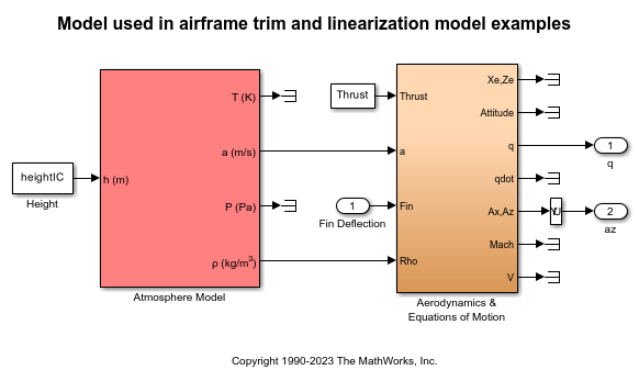
Initialize Guidance Model
Find the elevator deflection and the resulting trimmed body rate (q). These calculations generate a given incidence value when the airframe is traveling at a set speed. Once the trim condition is found, a linear model can be derived for the dynamics of the perturbations in the states around the trim condition.
open_system('aeroblk_guidance_airframe');
Define State Values
Define the state values for trimming:
Height [m]
Mach Number
Incidence [rad]
Flightpath Angle [rad]
Total Velocity [m/s]
Initial Pitch Body Rate [rad/sec]
heightIC    = 10000/m2ft;
machIC      = 3;
alphaIC     = -10*d2r;
thetaIC     = 0*d2r;
velocityIC  = machIC*(340+(295-340)*heightIC/11000);
pitchRateIC = 0;
Find Names and Ordering of States
Find the names and the ordering of states from the model.
[sizes,x0,names]=aeroblk_guidance_airframe([],[],[],'sizes');

state_names = cell(1,numel(names));
for i = 1:numel(names)
    n = max(strfind(names{i},'/'));
    state_names{i}=names{i}(n+1:end);
end
Specify States
Specify which states to trim and which states remain fixed.
fixed_states            = [{'U,w'} {'Theta'} {'Position'}];
fixed_derivatives       = [{'U,w'} {'q'}];
fixed_outputs           = [];
fixed_inputs            = [];

n_states=[];n_deriv=[];
for i = 1:length(fixed_states)
    n_states=[n_states find(strcmp(fixed_states{i},state_names))]; %#ok<AGROW>
end
for i = 1:length(fixed_derivatives)
    n_deriv=[n_deriv find(strcmp(fixed_derivatives{i},state_names))]; %#ok<AGROW>
end
n_deriv=n_deriv(2:end);                          % Ignore U
Trim Model
Trim the model.
[X_trim,U_trim,Y_trim,DX]=trim('aeroblk_guidance_airframe',x0,0,[0 0 velocityIC]', ...
                               n_states,fixed_inputs,fixed_outputs, ...
                               [],n_deriv)  %#ok<NOPTS>
X_trim =

   1.0e+03 *

   -0.0002
         0
    0.9677
   -0.1706
         0
   -3.0480


U_trim =

    0.1362


Y_trim =

   -0.2160
         0


DX =

         0
   -0.2160
  -14.0977
         0
  967.6649
 -170.6254
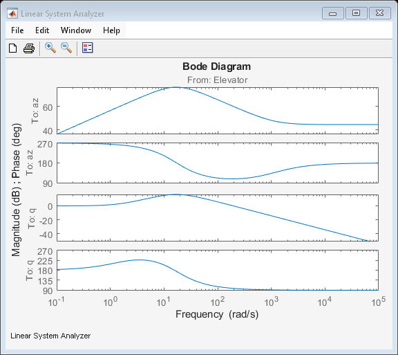
Linear Model and Frequency Response
Derive the linear model and view the frequency response.
[A,B,C,D]=linmod('aeroblk_guidance_airframe',X_trim,U_trim);
if exist('control','dir')
    airframe = ss(A(n_deriv,n_deriv),B(n_deriv,:),C([2 1],n_deriv),D([2 1],:));
    set(airframe,'StateName',state_names(n_deriv), ...
        'InputName',{'Elevator'}, ...
        'OutputName',[{'az'} {'q'}]);

    zpk(airframe)
    linearSystemAnalyzer('bode',airframe)
end
ans =

  From input "Elevator" to output...
          -170.45 s (s+1133)
   az:  ----------------------
        (s^2 + 30.04s + 288.9)

         -194.66 (s+1.475)
   q:  ----------------------
       (s^2 + 30.04s + 288.9)

Continuous-time zero/pole/gain model.
Copyright 1990-2023 The MathWorks, Inc.
See Also
Blocks
Functions
zpk(Control System Toolbox)
You can also select a web site from the following list:
Americas
- América Latina (Español)
- Canada (English)
- United States (English)
Europe
- Belgium (English)
- Denmark (English)
- Deutschland (Deutsch)
- España (Español)
- Finland (English)
- France (Français)
- Ireland (English)
- Italia (Italiano)
- Luxembourg (English)
- Netherlands (English)
- Norway (English)
- Österreich (Deutsch)
- Portugal (English)
- Sweden (English)
- Switzerland
- United Kingdom (English)